Second order tensors can be represented by matrices: \[
{\underset{\tilde{}}{\mathbf{F}}}=
\begin{pmatrix}
F_{11} & F_{12} & F_{13} \\
F_{21} & F_{22} & F_{23} \\
F_{31} & F_{32} & F_{33} \\
\end{pmatrix}
\]
In TFEL/MFront, a tensor is stored as an array of
values, as follows in \(3D\): \[
\underline{s}=
\begin{pmatrix}
s_{\,11}\quad
s_{\,22}\quad
s_{\,33}\quad
s_{\,12}\quad
s_{\,21}\quad
s_{\,13}\quad
s_{\,31}\quad
s_{\,23}\quad
s_{\,32}
\end{pmatrix}^{T}
\]
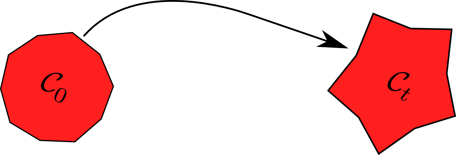
at a given time \(t\), a structure
is characterised by its {} \(\mathcal{C}_{t}\);
the initial configuration \(\mathcal{C}_{0}\) is often taken as the
reference configuration
the motion is described by a family of mappings \(\phi_{t}\), the {}, which associates a
point \(\vec{X}\) in \(\mathcal{C}_{0}\) to its position \(\vec{x}\) in \(\mathcal{C}_{t}\): \[
\vec{x}=\phi_{t}\left(\vec{X}\right)=\vec{X}+\vec{u}_{t}\left(\vec{X}\right)
\]
\(\vec{u}_{t}\) is the {}
Deformation gradient
Locally, the material is mechanically loaded if the deformation of
the current point differs from the deformation of its neighbours
The expansion of the deformation leads to: \[
\phi\left(\vec{X}+{{\mathrm{d}}}\,\vec{X}\right)-\phi\left(\vec{X}\right)={\displaystyle
\frac{\displaystyle \partial \phi}{\displaystyle \partial
\vec{X}}}\,.{{\mathrm{d}}}\,\vec{X}+\underbrace{\vec{X}\,.\,{{\displaystyle
\frac{\displaystyle \partial^{2}\,\phi}{\displaystyle
\partial\,\vec{X}^{2}}}}\,.{{\mathrm{d}}}\,\vec{X}+\ldots}_{\text{Higher
order terms}}
\]
The deformation gradient \({\underset{\tilde{}}{\mathbf{F}}}\) is a
tensor defined by: \[
{\underset{\tilde{}}{\mathbf{F}}}={\displaystyle \frac{\displaystyle
\partial \phi}{\displaystyle \partial
\vec{X}}}={\underset{\tilde{}}{\mathbf{I}}}+{\displaystyle
\frac{\displaystyle \partial \vec{u}}{\displaystyle \partial \vec{X}}}
\]
Higher order theories will not be considered in this course or in
this paper.
Polar decomposition
of \({\underset{\tilde{}}{\mathbf{F}}}\)
Polar decomposition
(Wikipedia)
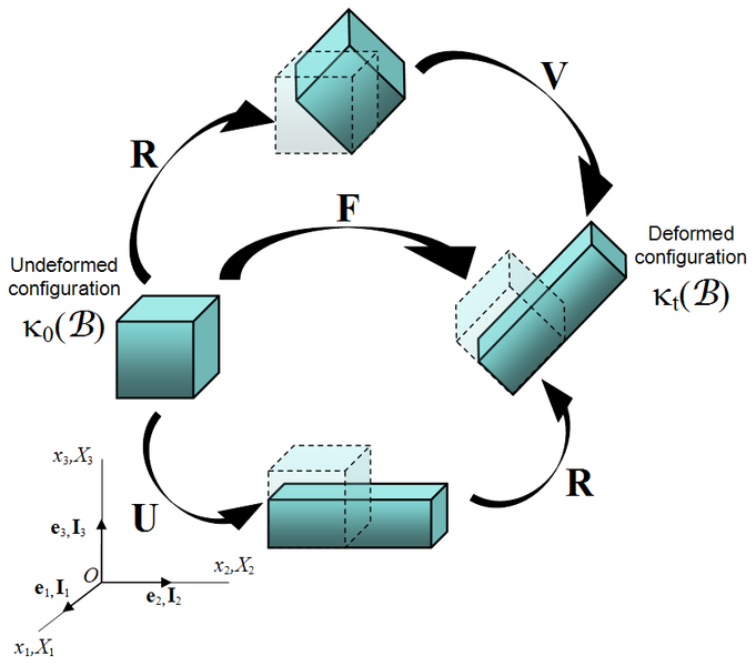
Uniqueness and existence of a polar decomposition of \({\underset{\tilde{}}{\mathbf{F}}}\): \(\quad\quad{\underset{\tilde{}}{\mathbf{F}}}={\underset{\tilde{}}{\mathbf{R}}}\,.\underline{U}=\underline{V}\,.{\underset{\tilde{}}{\mathbf{R}}}\)
\({\underset{\tilde{}}{\mathbf{R}}}\) is a
rotation
\(\underline{V}\) and \(\underline{U}\) are {}
\(\underline{V}\) is the eulerian
stretch tensor:
\(\left.\underline{V}\right|_{t}\)
and \(\left.\underline{V}\right|_{t+\Delta\,t}\)
are expressed in two different configurations:
\(\Delta\,\underline{V}=\left.\underline{V}\right|_{t+\Delta\,t}-\left.\underline{V}\right|_{t}\)
is {} well defined
\(\underline{U}\) is the lagrangian
stretch tensor:
expressed in the reference configuration
\(\Delta\,\underline{U}=\left.\underline{U}\right|_{t+\Delta\,t}-\left.\underline{U}\right|_{t}\)
is {}
\(\displaystyle\log\left({{\displaystyle
\frac{\displaystyle l\left(t\right)}{\displaystyle
l_{0}}}}\right)\) is sometimes called the true strain, although
the meaning of this is dubious, as discussed later
The expression \(\displaystyle\int_{l_{0}}^{l\left(t\right)}{{\displaystyle
\frac{\displaystyle {{\mathrm{d}}}\,l}{\displaystyle l}}}\) is
sometimes used to justify an incremental framework of the mechanics of
deformable body at finite strain (updated lagrangian formulations,
hypoelasticity): it’s a common pitfall of the \(80's\) which is still present in major
finite element solvers.
Mechanical equilibrium
Cauchy stress
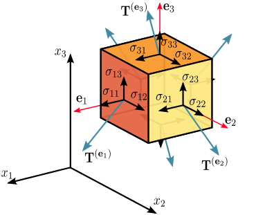
Components of the Cauchy stress
(Wikipedia)
The stress state of a body at a given point is characterised by a
second order tensor called the Cauchy stress: \(\quad\quad\quad\underline{\sigma}=
\begin{pmatrix} \sigma_{11} & \sigma_{12} & \sigma_{13}
\\ \sigma_{21} & \sigma_{22} & \sigma_{23} \\ \sigma_{31}
& \sigma_{32} & \sigma_{33} \end{pmatrix}\)
The Cauchy stress satisfies:\ \(\quad\quad\quad{{\mathrm{d}}}\vec{T} =
\underline{\sigma}\,.\,{{\mathrm{d}}}\vec{s}\)
\({{\mathrm{d}}}\vec{s}\): oriented
unit surface
\({{\mathrm{d}}}\vec{T}\): traction
acting on \({{\mathrm{d}}}\vec{s}\)
\({{\mathrm{d}}}\vec{s}\) is
defined in the current configuration
Example of a pressure \(p\) applied
to the boundary of a body, \(\vec{n}\)
being the outer normal to the boundary: \[
\underline{\sigma}\,.\,{{\mathrm{d}}}\vec{n}=-p
\]
Power of body forces: \[
\begin{aligned}
\int_{\Omega}\vec{f}\,.\,\vec{v}\,{{\mathrm{d}}}\,v
&=-\int_{\partial\,\Omega}\left(\underline{\sigma}\,.\,\vec{n}\right)\,.\,\vec{v}\,{{\mathrm{d}}}\,s+\int_{\Omega}\underline{\sigma}\,\colon\,{\underset{\tilde{}}{\mathbf{L}}}\,{{\mathrm{d}}}\,v\\
&=-\int_{\partial\,\Omega}\left(\underline{\sigma}\,.\,\vec{n}\right)\,.\,\vec{v}\,{{\mathrm{d}}}\,s+\int_{\Omega}\underline{\sigma}\,\colon\,{\underset{\tilde{}}{\mathbf{D}}}\,{{\mathrm{d}}}\,v\quad\text{(symmetry
of \(\underline{\sigma}\))}\\
\end{aligned}
\]
Hencky strain: \[\underline{\epsilon}^{\mathrm{to}}_{\mathrm{log}}=\log\underline{U}=\displaystyle\sum_{i=0}^{3}\log\lambda_{i}\,\underline{n}_{i}\]
where \(\lambda_{i}\) are the
eigenvalues of \(\underline{U}\) and
\(\underline{n}_{i}\) are its
eigentensors
functions of \({\underset{\tilde{}}{\mathbf{V}}}\) will
not be considered {}
\(\underline{\epsilon}^{\mathrm{to}}\) is {}
a strain measure, \({\underset{\tilde{}}{\mathbf{F}}}\) is {} a
strain measure
\({\underset{\tilde{}}{\mathbf{D}}}\) is {}
the time derivative of a strain measure
For each strain measure \(\underline{\epsilon}^{\mathrm{to}}_{\star}\),
one may define its dual stress \({\underset{\tilde{}}{\mathbf{T}}}_{\star}\):
\[
J\,\underline{\sigma}\,\colon\,\underline{D}=\underline{\tau}\,\colon\,\underline{D}=\underline{\epsilon}^{\mathrm{to}}_{\star}\,\colon\,{\underset{\tilde{}}{\mathbf{T}}}_{\star}
\]
The tensor \(\underline{\tau}=J\,\underline{\sigma}\) is
called the Kirchhoff stress.
The dual of the Green-Lagrange strain is the second Piola-Kirchhoff
stress \(\underline{S}\): \[
\underline{S}={\underset{\tilde{}}{\mathbf{F}}}^{-1}\,.\,\underline{\tau}\,.\,{\underset{\tilde{}}{\mathbf{F}}}^{-T}
\quad\Leftrightarrow\quad\tau =
{\underset{\tilde{}}{\mathbf{F}}}\,.\,\underline{S}\,.\,{\underset{\tilde{}}{\mathbf{F}}}^{T}
\]
There is no strain measure which is the dual of \(\underline{\tau}\), nor \(\underline{\sigma}\)
Choice of a stress/strain
couple
All strain measures are {}: there is no theoretical reason to prefer
one strain measure over another.
However, there are {} reasons to do so.
The Green-Lagrange strain
The Green-Lagrange strain and its dual are:
easy to compute (no computational penalty);
there is no straight-forward relation between the Green-Lagrange
strain and the change of volume - for small strain however: \[
J \approx
1+\mathrm{tr}\left(\underline{\epsilon}^{\mathrm{to}}_{\mathrm{GL}}\right)
\] \begin{center}
The Green-Lagrange strain framework is indeed well suited for
extending behaviours identified in the infinitesimal perturbation theory
to finite rotation*
The logarithmic strain
framework
There is a straight-forward relation between the Hencky strain
strain and the change of volume: \[
J =
\exp\left(\mathrm{tr}\left(\underline{\epsilon}^{\mathrm{to}}_{\mathrm{log}}\right)\right)
\]
\(\underline{T}_{\mathrm{log}}\) is
equal to the Kirchhoff stress \(\underline{\tau}\), which is equal to the
Cauchy stress \(\underline{\sigma}\)
for isochoric deformation
However, the Hencky strain and its dual are costly to compute (see
Miehe et al., 2005);
** The logarithmic strain framework is indeed well suited for
plasticity and/or viscoplasticity **
Elasticity
The mechanical work during the deformation process is (time integral
of the mechanical power): \[
w\left(0,t\right)=\int_{0}^{t}J\,\underline{\sigma}\,\colon\,\underline{D}\,{{\mathrm{d}}}\,t
=\int_{0}^{t}\underline{T}_{\star}\,\colon\,\underline{\epsilon}^{\mathrm{to}}_{\star}\,{{\mathrm{d}}}\,t
=\int_{\left.\underline{\epsilon}^{\mathrm{to}}_{\star}\right|0}^{\left.\underline{\epsilon}^{\mathrm{to}}_{\star}\right|t}\underline{T}_{\star}\,\colon\,{{\mathrm{d}}}\,\underline{\epsilon}^{\mathrm{to}}_{\star}
\]
Elasticity assumes that the previous integral is path-independent,
i.e. the mechanical work only depends on the current state of
deformation and not the history of the deformation process
The dual stress \(\underline{T}_{\star}\) then satisfies :
\[
\underline{T}_{\star} = {\displaystyle \frac{\displaystyle \partial
w}{\displaystyle \partial \underline{\epsilon}^{\mathrm{to}}_{\star}}}
\]
Linear Elasticity
Linear elasticity assumes a linear relationship between \(\underline{\epsilon}^{\mathrm{to}}_{\star}\)
and \(\underline{T}_{\star}\): \[
\underline{T}_{\star} =
\underset{=}{\mathbf{D}}\,\colon\,\underline{\epsilon}^{\mathrm{to}}_{\star}\quad\Leftrightarrow\quad
w={{\displaystyle \frac{\displaystyle 1}{\displaystyle
2}}}\underline{\epsilon}^{\mathrm{to}}_{\star}\,\colon\,\underset{=}{\mathbf{D}}\,\colon\,\underline{\epsilon}^{\mathrm{to}}_{\star}
\]
The fourth order tensor \(\underset{=}{\mathbf{D}}\) satisfies: \[
\underset{=}{\mathbf{D}}={{\displaystyle \frac{\displaystyle
\partial^{2}w}{\displaystyle
\partial\underline{\epsilon}^{\mathrm{to}}_{\star}\partial\underline{\epsilon}^{\mathrm{to}}_{\star}}}}
\]
\(\underset{=}{\mathbf{D}}\) have
the following properties:
\(\underset{=}{\mathbf{D}}\) has
minor symmetries (\(\underline{T}_{\star}\) and \(\underline{\epsilon}^{\mathrm{to}}_{\star}\)
are symmetric): \[
D_{ijkl}= D_{jikl}\quad\text{and}\quad D_{ijkl}= D_{ijlk}
\]
\(\underset{=}{\mathbf{D}}\) has
major symmetries (Schwarz theorem): \[
D_{ijkl}=D_{klij}
\]
Isotropic elasticity
For an isotropic material, only two independant material properties
remains: \[
\underline{T}_{\star}
=
\lambda\,\left(\mathrm{tr}\left(\underline{\epsilon}^{\mathrm{to}}_{\star}\right)\right)\,\underline{I}+2\,\mu\,\underline{\epsilon}^{\mathrm{to}}_{\star}
\]
\(\lambda\) and \(\mu\) are called the Lamé coefficients
\(\mu\) is also called the shear
modulus
In the infinitesimal perturbation hypothesis, this is the Hooke
law.
In the Green-Lagrange strain framework, this is the Saint-Venant
Kirchhoff law.
In the logarithmic strain framework, this is the Hencky-Biot
law.
Bulk modulus
Separate change of volume from deviatoric part: \[
\begin{aligned}
\underline{T}_{\star}&=
\lambda\,\left(\mathrm{tr}\left(\underline{\epsilon}^{\mathrm{to}}_{\star}\right)\right)\,\underline{I}+2\,\mu\,\underline{\epsilon}^{\mathrm{to}}_{\star}
\\
&= \left(\lambda+{{\displaystyle \frac{\displaystyle
2\,\mu}{\displaystyle
3}}}\right)\,\underbrace{\left(\mathrm{tr}\left(\underline{\epsilon}^{\mathrm{to}}_{\star}\right)\right)\,\underline{I}}_{\text{volume
change}}+2\,\mu\,\underbrace{\left(\underline{\epsilon}^{\mathrm{to}}_{\star}-{{\displaystyle
\frac{\displaystyle
\mathrm{tr}\left(\underline{\epsilon}^{\mathrm{to}}_{\star}\right)}{\displaystyle
3}}}\,\underline{I}\right)}_{\text{deviator}} \\
&=
K\,\left(\mathrm{tr}\left(\underline{\epsilon}^{\mathrm{to}}_{\star}\right)\right)\,\underline{I}+2\,\mu\,\left(\underline{\epsilon}^{\mathrm{to}}_{\star}-{{\displaystyle
\frac{\displaystyle
\mathrm{tr}\left(\underline{\epsilon}^{\mathrm{to}}_{\star}\right)}{\displaystyle
3}}}\,\underline{I}\right) \\
\end{aligned}
\]
\(K=\lambda+{{\displaystyle
\frac{\displaystyle 2\,\mu}{\displaystyle 3}}}\) is called the
bulk modulus
The total strain is splitted into an elastic part and a thermal
part: \[
\underline{\epsilon}^{\mathrm{to}}_{\star}=
\underline{\epsilon}^{\mathrm{el}}_{\star}+
\underline{\epsilon}^{\mathrm{th}}_{\star}
\]
The elastic part \(\underline{\epsilon}^{\mathrm{el}}_{\star}\)
defines the stresses \(\underline{T}_{\star}\) through the Hooke
law: \[
\underline{T}_{\star}=\underset{=}{\mathbf{D}}\,\colon\,\underline{\epsilon}^{\mathrm{el}}_{\star}
\]
Isotropic thermal expansion
The thermal expansion is given by: \[
{{\displaystyle \frac{\displaystyle \Delta\,l}{\displaystyle
l_{T^{\alpha}}}}}={{\displaystyle \frac{\displaystyle
l_{T}-l_{T^{\alpha}}}{\displaystyle
l_{T^{\alpha}}}}}=\alpha\left(T\right)\,\left(T-T^{\alpha}\right)
\]
If the reference temperature \(T^{\alpha}\) for the thermal expansion is
different than the reference temperature \(T^{i}\) of the geometry: \[
{{\displaystyle \frac{\displaystyle \Delta\,l}{\displaystyle
l_{T^{i}}}}} = {{\displaystyle \frac{\displaystyle 1}{\displaystyle
1+\alpha\left(T^{i}\right)\,\left(T^{i}-T^{\alpha}\right)}}}\,\left[\alpha\left(T\right)\,\left(T-T^{\alpha}\right)-\alpha\left(T^{i}\right)\,\left(T^{i}-T^{\alpha}\right)\right]
\]
Isotropic damage
Visco-plasticity
A first approach to
viscoplastic behaviour
The total strain is splitted into an elastic part and a viscoplastic
part: \[
\underline{\epsilon}^{\mathrm{to}}_{\star}=
\underline{\epsilon}^{\mathrm{el}}_{\star}+
\underline{\epsilon}^{\mathrm{vis}}_{\star}
\]
The plastic flow is generally isochoric: \[
\mathrm{tr}\left(\underline{\epsilon}^{\mathrm{vis}}_{\star}\right)=0
\]
Without internal state, the mechanical dissipation associated with
plasticity is: \[
\underline{T}_{\star}\,\colon\,\underline{\dot{\epsilon}}^{\mathrm{tox}}_{\star}=
\underbrace{\underline{T}_{\star}\,\colon\,\underline{\dot{\epsilon}}^{\mathrm{el}}_{\star}}_{\text{stored
reversibly}}+
\underbrace{\underline{T}_{\star}\,\colon\,\underline{\dot{\epsilon}}^{\mathrm{vis}}_{\star}}_{\text{dissipated}}
\]
The expression dissipated power can be rewritten using the deviator
of the stress \(\underline{s}_{\star}\): \[
\underline{T}_{\star}\,\colon\,\underline{\dot{\epsilon}}^{\mathrm{vis}}_{\star}=
\underline{s}_{\star}\,\colon\,\underline{\dot{\epsilon}}^{\mathrm{vis}}_{\star}
\quad\text{with}\quad\underline{s}_{\star}=\underline{T}_{\star}-{{\displaystyle
\frac{\displaystyle 1}{\displaystyle
3}}}\,\mathrm{tr}\left(\underline{T}_{\star}\right)\,\underline{I}
\]
The dissipation is maximal if the \(\underline{\dot{\epsilon}}^{\mathrm{vis}}_{\star}\)
is colinear with \(\underline{s}_{\star}\).
The Von Mises stress
The material is now assumed {}
A convenient isotropic norm for deviatoric stress tensor is the Von
Mises norm: \[
T^{eq}_{\star}=\sqrt{{{\displaystyle \frac{\displaystyle
3}{\displaystyle
2}}}\underline{s}_{\star}\,\colon\,\underline{s}_{\star}}
\]
The \({{\displaystyle \frac{\displaystyle
3}{\displaystyle 2}}}\) factor is here so that in uniaxial
tensile tests: \[
T^{eq}_{\star}=\left|T_{xx}\right|
\]
The Von Mises norm is one the three invariants of the stress (the
other ones are the pressure and the determinant)
In term of eigen values: \[
T^{eq}_{\star}=\sqrt{{{\displaystyle \frac{\displaystyle
1}{\displaystyle
2}}}\left[\left(T_{1}-T_{2}\right)^{2}+\left(T_{1}-T_{3}\right)^{2}+\left(T_{2}-T_{3}\right)^{2}\right]}
\]
The normal tensor
The equation: \[
T^{eq}_{\star}=\text{Cste}
\] defines a sphere in the deviatoric space
The normal to this surface is: \[
\underline{n}_{\star}={\displaystyle \frac{\displaystyle \partial
T^{eq}_{\star}}{\displaystyle \partial
\underline{T}_{\star}}}={{\displaystyle \frac{\displaystyle
3\,\underline{s}_{\star}}{\displaystyle 2\,T^{eq}_{\star}}}}
\]
The normal is colinear to \(\underline{s}_{\star}\), thus an isochoric
viscoplastic flow of the form: \[
\underline{\dot{\epsilon}}^{\mathrm{vis}}_{\star}=f\left(\underline{T}_{\star}\right)\underline{n}_{\star}
\] would maximise the mechanical dissipation.
The viscoplastic flow is: \(\underline{\dot{\epsilon}}^{\mathrm{vis}}_{\star}=f\left(\underline{T}_{\star}\right)\underline{n}_{\star}\)
The material being isotropic, \(f\)
must be a function of the invariants of the stresses: the pressure, the
Von Mises stress, the determinant.
Experimentally, viscoplastic behaviour is found to be pressure
insensitive.
The effect of the third invariant is neglected in general.
Thus, a simple viscoplastic model for an isotropic incompressible
material is: \[
\underline{\dot{\epsilon}}^{\mathrm{vis}}_{\star}=f\left(T^{eq}_{\star}\right)\underline{n}_{\star}
\]
Restrictions:
\(f\) must be positive for the
dissipation to be positive
\(f\left(\underline{0}\right)\)
must be null
The Norton behaviour correspond to a power function: \[
\underline{\dot{\epsilon}}^{\mathrm{vis}}_{\star}=A\,\left(T^{eq}_{\star}\right)^{n}\underline{n}_{\star}=\dot{\varepsilon}^{0}\left({{\displaystyle
\frac{\displaystyle T^{eq}_{\star}}{\displaystyle
T^{0}}}}\right)^{n}\underline{n}_{\star}
\]
Equivalent viscoplastic
strain
A convenient choice for the viscoplastic strain rate norm is: \[
\dot{p}=f\left(T^{eq}_{\star}\right)=\sqrt{{{\displaystyle
\frac{\displaystyle 2}{\displaystyle
3}}}\,\underline{\dot{\epsilon}}^{\mathrm{vis}}_{\star}\,\colon\,\underline{\dot{\epsilon}}^{\mathrm{vis}}_{\star}}
\]
In uniaxial tensile tests: \[
\dot{p} =
\left|\left(\dot{\epsilon}^{\mathrm{vis}}_{\star}\right)_{xx}\right|
\]
The equivalent viscoplastic strain is defined by: \[
p=\int_{0}^{t}\dot{p}\,{{\mathrm{d}}}\,t
\]
This quantity is a convenient measure of the viscoplastic history of
the material and is widely used as a damage criterium.
Dissipation potential
The Norton behaviour can be expressed as: \[
\underline{\dot{\epsilon}}^{\mathrm{vis}}_{\star}={\displaystyle
\frac{\displaystyle \partial \Phi^{\star}}{\displaystyle \partial
\underline{T}_{\star}}}
\quad\text{with}\quad
\Phi^{\star}\left(T^{eq}_{\star}\right)={{\displaystyle
\frac{\displaystyle T^{0}\dot{\varepsilon}^{0}}{\displaystyle
n+1}}}\left({{\displaystyle \frac{\displaystyle
T^{eq}_{\star}}{\displaystyle T^{0}}}}\right)^{n+1}
\]
\(\Phi^{\star}\) is called the
dissipation potential
Other expressions of the dissipation potential defines used the
define other viscoplastic behaviours.
The resulting viscoplastic behaviours will lead to a positive
dissipation if \(\Phi^{\star}\) is {}
and {} at zero.
The introduction of dissipation potentials is the departure of a
theorical developments which can ease the formulation of mechanical
behaviours:
thermodynamical consistent behaviours
numerically efficient behaviours
Thermodynamics
First principle
The Finite Element Method
Principle of virtual power
Let \(\partial_{u}\Omega\) the
boundary part where displacements are prescribed
\(\partial_{t}\Omega=\partial\Omega\setminus\partial_{u}\Omega\)
is the boundary part where tractions are prescribed
Let \(\vec{v}^{\star}\) be a vector
field compatible with prescribed displacement and \(\delta\,\vec{v}^{\star}=\vec{v}^{\star}-\vec{v}\),
then: \[
\underbrace{\int_{\Omega}\underline{\sigma}\,\colon\,\delta\,{\underset{\tilde{}}{\mathbf{D}}}^{\star}\,{{\mathrm{d}}}\,v}_{\text{virtual
inner forces power}} =
\underbrace{\int_{\Omega}\vec{f}\,.\,\delta\,\vec{v}^{\star}\,{{\mathrm{d}}}\,v
+
\int_{\partial\,\Omega_{t}}\vec{t}\,.\,\delta\,\vec{v}^{\star}\,{{\mathrm{d}}}\,s}_{\text{virtual
external forces power}}
\]
this is the principle of virtual power which is the basis of the
Finite Element Method (FEM)
Finite element method
The principle of virtual power is used to find the best
approximation of the solution on a finite space.
Finite elements are a widely used way of defining such a finite
space by discretizing the real geometry by subdomains called finite
elements:
Given values at specified points of the finite element (the nodes),
the function value is approximated by interpolation functions.
Resolution
Mechanical equilibrium: find\(\Delta\mathbb{\vec{u}}\) such as: \[
\small
\mathbb{\vec{R}}\left(\Delta\mathbb{\vec{u}}\right)=\mathbb{\vec{O}}\quad\text{
avec
}\quad\mathbb{\vec{R}}\left(\Delta\mathbb{\vec{u}}\right)=\mathbb{\vec{F}}_{i}\left(\Delta\mathbb{\vec{u}}\right)-\mathbb{\vec{F}}_{e}
\]
element contribution to inner forces: \[
\small
\begin{aligned}
\mathbb{\vec{F}}_{i}^{e}&=\int_{V^{e}}\underline{\sigma}_{t+\Delta
t}\left(\Delta\,\underline{\epsilon}^{\mathrm{to}},\Delta\,
t\right)\colon\underline{B}\;{{\mathrm{d}}}V \\
&= \sum_{i=1}^{N^{G}}
\left(\underline{\sigma}_{t+\Delta\,t}\left(\Delta\underline{\epsilon}^{\mathrm{to}}\left(\vec{\eta}_{i}\right),\Delta\,
t\right)\colon\underset{=}{\mathbf{B}}\left(\vec{\eta}_{i}\right)\right)w_{i}
\end{aligned}
\] where \(\underline{B}\) gives
the relationship between \(\Delta\,\underline{\epsilon}^{\mathrm{to}}\)
and \(\Delta\mathbb{\vec{u}}\)