Introduction

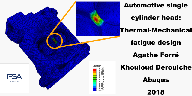
MFront version 3.0 provides two interfaces for the Abaqus/Standard and Abaqus/Explicit finite element solvers. Those interfaces are fairly features complete:

• Isotropic and orthotropic materials are supported.
• Small and finite strain behaviours are supported.

It shall be pointed out that the Abaqus/Standard and Abaqus/Explicit solvers have a long history. In particular, the design choices made for the UMAT and VUMAT interfaces were meant to allow the users to easily write finite-strain behaviours in rate-form. However, their choices differ in many points. As a consequence, those interfaces are not compatible “out of the box”: i.e. one cannot restart a simulation with Abaqus/Explicit after a computation with Abaqus/Standard without precautions.

MFront strives to provides behaviours that can be used “just-like” other UMAT and VUMAT subroutines, but there are some cases (namely finite strain orthotropic behaviours) where we were obliged to make some unusual choices that are described in this document for various reasons:

• Ensure the compatibility between the Abaqus/Standard and Abaqus/Explicit.
• Have optimal performances.

Pitfalls

There are also cases of misuses of the generated libraries that can not be prevented by MFront. The most important ones are the following:

• For Abaqus/Standard, small strain isotropic behaviour can be used in finite strain analyses “out of the box.” However, if a behaviour is meant to be used only for finite strain analyses, we recommend using one one of the finite strain strategies available (See the @AbaqusFiniteStrainStrategy keyword and the section dedicated to finite strain strategies below). The Native finite strain strategy will use the Abaqus/Standard functionalities to integrate the behaviour in “rate-form” and also adds a correction to the tangent operator (see below for details). The user must then be aware that when using the Native finite strain strategy, results will depend on the fact that an orientation is defined or not. Futhermore, behaviours using the Native finite strain strategy (or no strategy at all) can not be ported to other solver. If portability is an issue, consider using one of the other finite strain strategy (see below).
• For Abaqus/Standard, the usage of the Native finite strain strategy is not compatible with Abaqus/Explicit because the latter always uses a corotationnal frame associated with the Green-Nagdy objective derivative to integrate the behaviour in rate-form, when Abaqus/Standard uses a corotationnal frame associated with the Jaumann objective derivative.
• For Abaqus/Standard, the number of field variables (corresponding to external state variables in MFront) can not be checked.
• For Abaqus/Standard, one shall not combine the MFront orthotropy policy with the definition of an orientation.
• For Abaqus/Standard, one have to use the MFront orthotropy policy to handle orthotropic finite strain behaviours (see below for details).

Current status

These interfaces have been extensively tested through MTest. Tests on Abaqus/Standard and Abaqus/Explicit shows that MFront behaviours are efficient (to the extent allowed by the UMAT and VUMAT interfaces respectively) and reliable.

How the use MFront behaviours in Abaqus/Standard and Abaqus/Explicit

When compiling mechanical behaviours with the Abaqus/Standard and/or Abaqus/Explicit interfaces, MFront generates:

• shared libraries containing one implementation of the considered behaviours per supported modelling hypotheses.
• examples of input files in the abaqus or abaqus-explicit directory, respectively
• a copy of a generic umat.cpp file for the Abaqus/Standard solver
• a copy of generic vumat-sp.cpp (for single precision computation) and vumat-dp.cpp (for double precision computations) files for the Abaqus/Explicit solver

The user must launch Abaqus/Standard or Abaqus/Explicit with one of the previous generic files as an external user file. Those files handles the loading of MFront shared libraries using the material name: the name of the material shall thus define the function to be called and the library in which this function is implemented.

The function name includes the modelling hypothesis, see below. An identifier can optionnaly be added to reuse the same behaviour for several material (with different material properties for instance). The identifier is discarded in the umat.cpp, vumat-sp.cpp and and vumat-dp.cpp files.

Thus, the material name in Abaqus/Standard and Abaqus/Explicit is expected to have the following form: LIBRARY_FUNCTION_HYPOTHESIS_IDENTIFIER.

The first part is the name of library, without prefix (lib) or suffix (.dll or .so depending on the system). This convention implies that the library name does not contain an underscore character.

For example, on UNIX systems, if one want to call the ELASTICITY_3D behaviour in libABAQUSBEHAVIOUR.so library, the name of the material in the Abaqus/Standard input file has to be: ABAQUSBEHAVIOUR_ELASTICITY_3D.

This leads to the following declaration of the material:

*Material, name=ABAQUSBEHAVIOUR_ELASTICITY_3D

It is important to note that the name of the behaviour is automatically converted to upper-case by Abaqus/Standard or Abaqus/Explicit. The name of the libraries generated by MFront are thus upper-cased. The user shall thus be aware that he/she must not rename MFront generated libraries using lower-case letters.

Notes

• The MFront libraries are only generated once, only the generic files needs to be recompiled at each run. This is very handy since compiling the MFront libraries can be time-consuming. Those libraries can be shared between computations and/or between users when placed in a shared folders.
• The fact that MFront generates one implementation per modelling hypothesis allows the distinction between the plane strain hypothesis and the axisymmetrical hypothesis. This is mandatory to consistently handle orthotropy.
• The name of the library can be changed by renaming it after the compilation or by using the @Library keyword.

Note on libraries locations

As explained above, MFront libraries will be loaded at the runtime time. This means that the libraries must be found by the dynamic loader of the operating system.

Under Linux

Under Linux, the search path for dynamic libraries are specified using the LD_LIBRARY_PATH variable environment. This variable defines a colon-separated set of directories where libraries should be searched for first, before the standard set of directories.

Depending on the configuration of the system, the current directory can be considered by default.

Under Windows

Under Windows, the dynamic libraries are searched:

• in the current directory
• in the directories listed in the PATH environment. This variable defines a semicolon-separated set of directories.

Compilation of the generic umat.cpp or vumat-*.cpp files

Depending on the compiler and compiler version, appropriate flags shall be added for the compilation of the generic umat.cpp or vumat-*.cpp files which are written against the C++11 standard.

The procedure depends on the version of Abaqus used. In every case, one shall modify a file called abaqus_v6.env which is delivered with Abaqus. The modified version of this file must be in the current working directory.

Versions later than Abaqus 2017

In the abaqus_v6.env, one can load a specific environment file using the importEnv function:

# Import site specific parameters such as licensing and doc parameters
importEnv('<path>/custom_v6.env')

This file, called custom_v6.env, is used to modify the compile_cpp entry which contains the command line used to compile C++ files. The content of this file can be copied from one of the system specific environment file delivered with Abaqus. For example, under LinuX, one can use the lnx86_64.env as a basis to build the custom_v6.env.

Here is an example of a modified custom_v6.env (we changed several paths that must be updated to match your installation):

# Installation of Abaqus CAE 2017
# Mon Jul 17 15:06:17 2017
plugin_central_dir="/appli/abaqus/linuxo/V6R2017x/CAE/plugins"
doc_root="file:////usr/DassaultSystemes/SIMULIA2017doc/English"
license_server_type=FLEXNET
abaquslm_license_file="<licenfile>"
compile_cpp = ['g++', '-O2', '-std=c++11','-c', '-fPIC', '-w', '-Wno-deprecated', '-DTYPENAME=typename',
               '-D_LINUX_SOURCE', '-DABQ_LINUX', '-DABQ_LNX86_64', '-DSMA_GNUC',
               '-DFOR_TRAIL', '-DHAS_BOOL', '-DASSERT_ENABLED',
               '-D_BSD_TYPES', '-D_BSD_SOURCE', '-D_GNU_SOURCE',
               '-D_POSIX_SOURCE', '-D_XOPEN_SOURCE_EXTENDED', '-D_XOPEN_SOURCE',
               '-DHAVE_OPENGL', '-DHKS_OPEN_GL',  '-DGL_GLEXT_PROTOTYPES',
               '-DMULTI_THREADING_ENABLED', '-D_REENTRANT',
               '-DABQ_MPI_SUPPORT', '-DBIT64', '-D_LARGEFILE64_SOURCE', '-D_FILE_OFFSET_BITS=64', '%P',
               # '-O0', # <-- Optimization level
               # '-g',  # <-- Debug symbols
               '-I%I']
usub_lib_dir='<path_to_mfront_generated_libraries>:<path_to_mfront>/lib'

The last line define a set of paths where shared libraries will be searched for, which is useful if one does not want to install TFEL and MFront on in system wide path (such as /usr/) or modify the LD_LIBRARY_PATH environment variable. One can also specify a shared directory (on a NFS file system for example) to access material behaviours shared among a team of colleagues.

Versions prior to Abaqus v2017

The appropriate flags can be defined in the abaqus_v6.env file that can be overridden by the user.

For the gcc compiler, one have to add the --std=c++11 flag. The modifications to be made to the abaqus_v6.env are the following:

cppCmd  = "g++"     # <-- C++ compiler
compile_cpp = [cppCmd,
               '-c', '-fPIC', '-w', '-Wno-deprecated', '-DTYPENAME=typename',
               '-D_LINUX_SOURCE', '-DABQ_LINUX', '-DABQ_LNX86_64', '-DSMA_GNUC',
               '-DFOR_TRAIL', '-DHAS_BOOL', '-DASSERT_ENABLED',
               '-D_BSD_TYPES', '-D_BSD_SOURCE', '-D_GNU_SOURCE',
               '-D_POSIX_SOURCE', '-D_XOPEN_SOURCE_EXTENDED', '-D_XOPEN_SOURCE',
               '-DHAVE_OPENGL', '-DHKS_OPEN_GL',  '-DGL_GLEXT_PROTOTYPES',
               '-DMULTI_THREADING_ENABLED', '-D_REENTRANT',
               '-DABQ_MPI_SUPPORT', '-DBIT64', '-D_LARGEFILE64_SOURCE',
               '-D_FILE_OFFSET_BITS=64', '-O2', '-std=c++11',
               mpiCppImpl,'-I\%I']

Generated input files

Here is an extract of the generated input file for a MFront behaviour named Plasticity for the plane strain modelling hypothesis for the Abaqus/Standard solver:

** Example for the 'PlaneStrain' modelling hypothesis
*Material, name=ABAQUSBEHAVIOUR_PLASTICITY_PSTRAIN
*Depvar
5,
1, ElasticStrain_11
2, ElasticStrain_22
3, ElasticStrain_33
4, ElasticStrain_12
5, EquivalentPlasticStrain
** The material properties are given as if we used parameters to explicitly
** display their names. Users shall replace those declaration by
** theirs values and/or declare those parameters in the appropriate *parameters
** section of the input file
*User Material, constants=4
<YoungModulus>, <PoissonRatio>, <H>, <s0>

Main features

Supported behaviours

Isotropic and orthotropic behaviours are both supported.

For orthotropic behaviours, there are two orthotropy management policy (see the AbaqusOrthotropyManagementPolicy keyword):

• Native: an orientation must be defined
• MFront: no orientation must be defined. The material frame is defined through additional state variables.

For Abaqus/Standard, small and finite strain behaviours are supported. For orthotropic finite strain behaviours, one must use the MFront orthotropy management policy. The reason of this choices is given below.

For Abaqus/Explicit, only finite strain are supported. Small strain behaviours can be used using one of the finite strain strategies available.

Modelling hypotheses

The following modelling hypotheses are supported:

• tridimensional (3D)
• plane strain (PSTRAIN)
• plane stress (including shell elements) (PSTRESS)
• axisymmetrical (AXIS)

The generalised plane strain hypothesis is currently not supported.

The Abaqus/Standard interface

The Abaqus/Standard solver provides the UMAT interface. In this case, the behaviour shall compute:

• The evolution of the state variables.
• The value the Cauchy stress at the end of the time step.
• The consistent tangent operator. The definition of the consistent tangent operator is given below.

For finite strain analyses, small strain behaviours can be written in rate form. The behaviour in integrated in the Jauman framework. This is different from Abaqus/Explicit which uses a corotational basis based on the Green-Nagdi rate.

Finite strain behaviours and orthotropy management policy

Orthotropic finite strain behaviours are only supported using the MFront orthotropy management policy. In this case, all quantities are expressed in the global configuration. Rotation in the initial material frame is handled by MFront.

Finite strain strategies

Engineers are used to write behaviours based on an additive split of strains, as usual in small strain behaviours. Different strategies exist to:

• write finite strain behaviours that preserve this property.
• guarantee some desirable properties such as energetic consistency and objectivity.

Through the @AbaqusFiniteStrainStrategy, the user can select on of various finite strain strategies supported by MFront, which are described in this paragraph.

Note

The usage of the @AbaqusFiniteStrainStrategy keyword is mostly deprecated since MFront 3.1: see the @StrainMeasure keyword.

The Native finite strain strategy

Among them is the Native finite strain strategy which relies on build-in Abaqus/Standard facilities to integrate the behaviours written in rate form. The Native finite strain strategy will use the Jauman rate.

Those strategies have some theoretical drawbacks (hypoelasticity, etc…) and are not portable from one code to another.

Recommended finite strain strategies

Two other finite strain strategies are available in MFront for the Abaqus/Standard interface (see the @AbaqusFiniteStrainStrategy keyword):

• ‘FiniteRotationSmallStrain’: this finite strain strategy is fully described in [1],[3]
• ‘MieheApelLambrechtLogarithmicStrain’: this finite strain strategy is fully described in [4] and
  1. This finite strain strategy is yet to be implemented.

Those two strategies use lagrangian tensors, which automatically ensures the objectivity of the behaviour.

Each of these two strategies define an energetic conjugate pair of strain or stress tensors:

• For the ‘FiniteRotationSmallStrain’ case, the strain tensor is the Green-Lagrange strain and the conjugated stress is the second Piola-Kirchhoff stress.
• For the ‘MieheApelLambrechtLogarithmicStrain,’ the strain tensor is the langrangian Hencky strain tensor, i.e. the logarithm of the stretch tensor.

The first strategy is suited for reusing behaviours that were identified under the small strain assumptions in a finite rotation context. The usage of this behaviour is still limited to the small strain assumptions.

The second strategy is particularly suited for metals, as incompressible flows are characterized by a deviatoric logarithmic strain tensor, which is the exact transposition of the property used in small strain behaviours to handle plastic incompressibility. This means that all valid consistutive equations for small strain behaviours can be automatically reused in finite strain analysis. This does not mean that a behaviour identified under the small strain assumptions can be directly used in a finite strain analysis: the identification would not be consistent.

Those two finite strain strategies are fairly portable and are available (natively or via MFront) in Cast3M, Code_Aster, Europlexus and Zebulon, etc…

Consistent tangent operator for finite strain behaviours

The “Abaqus User Subroutines Reference Guide” indicates that the tangent moduli required by Abaqus/Standard \(\underline{\underline{\mathbf{C}}}^{MJ}\) is closely related to \(\underline{\underline{\mathbf{C}}}^{\tau\,J}\), the moduli associated to the Jauman rate of the Kirchhoff stress :

\[ J\,\underline{\underline{\mathbf{C}}}^{MJ}=\underline{\underline{\mathbf{C}}}^{\tau\,J} \]

where \(J\) is the determinant of the deformation gradient \({\underset{\tilde{}}{\mathbf{F}}}\).

By definition, \(\underline{\underline{\mathbf{C}}}^{\tau\,J}\) satisfies: \[ \overset{\circ}{\underline{\tau}}^{J}=\underline{\underline{\mathbf{C}}}^{\tau\,J}\,\colon\underline{D} \] where \(\underline{D}\) is the rate of deformation.

The Abaqus/Explicit interface

Using Abaqus/Explicit, computations can be performed using single (the default) or double precision. The user thus must choose the appropriate generic file for calling MFront behaviours:

• the vumat-sp.cpp file is used for single precision.
• the vumat-dp.cpp file is used for double precision.

For double precision computation, the user must pass the double=both command line arguments to Abaqus/Explicit so that both the packaging steps and the resolution are performed in double precision (by default, if only the double command line argument is passed to Abaqus/Explicit, the packaging step is performed in single precision and the resolution is performed in double precision).

It is important to carefully respect those instructions: otherwise, Abaqus/Explicit will crash due to a memory corruption (segmentation error).

Here is an example of Abaqus invocation:

Abaqus user=vumat-dp.cpp double=both job=...

Finite strain strategies

As for Abaqus/Standard, user may choose one of the finite strain strategies available through MFront.

The Native finite strain strategy

The Native finite strain strategy relies on build-in Abaqus/Explicit facilities to integrate the behaviours written in rate form, i.e. it will integrate the behaviour using a corotationnal approach based on the polar decomposition of the deformation gradient.

Recommended finite strain strategies

The other finite strain strategies described for Abaqus/Standard are also available for the Abaqus/Explicit interface:

• ‘FiniteRotationSmallStrain’
• ‘MieheApelLambrechtLogarithmicStrain’

Energies

MFront behaviours can optionally compute the stored and dissipated energies through the @InternalEnergy and @DissipatedEnergy keywords.

In Abaqus/Standard, the stored energy is returned in the SSE output and the dissipated energy is returned in the SPD output.

In Abaqus/Explicit, the stored energy is returned in the enerInternNew variable and the the dissipated energy is returned in the enerInelasNew output.

A

Appendix

Most information reported here are extracted from the book of Belytschko ([5]).

Relations between tangent operator

Relation with the moduli associated to the Truesdell rate of the Cauchy Stress \(\underline{\underline{\mathbf{C}}}^{\sigma\,T}\)

The moduli associated to the Truesdell rate of the Cauchy Stress \(\underline{\underline{\mathbf{C}}}^{\sigma\,T}\) is related to \(\underline{\underline{\mathbf{C}}}^{\tau\,J}\) by the following relationship:

\[ \underline{\underline{\mathbf{C}}}^{\tau\,J}=J\,\left(\underline{\underline{\mathbf{C}}}^{\sigma\,T}+\underline{\underline{\mathbf{C}}}^{\prime}\right)\quad\text{with}\quad\underline{\underline{\mathbf{C}}}^{\prime}\colon\underline{D}=\underline{\sigma}\,.\,\underline{D}+\underline{D}\,.\,\underline{\sigma} \]

Thus,

\[ \underline{\underline{\mathbf{C}}}^{MJ}=\underline{\underline{\mathbf{C}}}^{\sigma\,T}+\underline{\underline{\mathbf{C}}}^{\prime} \]

Relation with the spatial moduli \(\underline{\underline{\mathbf{C}}}^{s}\)

The spatial moduli \(\underline{\underline{\mathbf{C}}}^{s}\) is associated to the Lie derivative of the Kirchhoff stress \(\mathcal{L}\underline{\tau}\) , which is also called the convected rate or the Oldroyd rate:

\[ \mathcal{L}\underline{\tau}=\underline{\underline{\mathbf{C}}}^{s}\,\colon\,\underline{D} \]

The spatial moduli is related to the moduli associated to Truesdell rate of the Cauchy stress \(\underline{\underline{\mathbf{C}}}^{\sigma\,T}\):

\[ \underline{\underline{\mathbf{C}}}^{\sigma\,T}=J^{-1}\,\underline{\underline{\mathbf{C}}}^{s} \]

Thus, we have: \[ \underline{\underline{\mathbf{C}}}^{MJ}= J^{-1}\underline{\underline{\mathbf{C}}}^{s}+\underline{\underline{\mathbf{C}}}^{\prime} = J^{-1}\left(\underline{\underline{\mathbf{C}}}^{s}+\underline{\underline{\mathbf{C}}}^{\prime\prime}\right)\quad\text{with}\quad\underline{\underline{\mathbf{C}}}^{\prime\prime}\colon\underline{D}=\underline{\tau}\,.\,\underline{D}+\underline{D}\,.\,\underline{\tau} \]

Relation with \(\underline{\underline{\mathbf{C}}}^{\mathrm{SE}}\)

The \(\underline{\underline{\mathbf{C}}}^{\mathrm{SE}}\) relates the rate of the second Piola-Kirchhoff stress \(\underline{S}\) and the Green-Lagrange strain rate \(\underline{\varepsilon}^{\mathrm{GL}}\):

\[ \underline{\dot{S}}=\underline{\underline{\mathbf{C}}}^{\mathrm{SE}}\,\colon\,\underline{\dot{\varepsilon}}^{\mathrm{GL}} \]

As the Lie derivative of the Kirchhoff stress \(\mathcal{L}\underline{\tau}\) is the push-forward of the second Piola-Kirchhoff stress rate \(\underline{\dot{S}}\) and the rate of deformation \(\underline{D}\) is push-forward of the Green-Lagrange strain rate \(\underline{\dot{\varepsilon}}^{\mathrm{GL}}\), \(\underline{\underline{\mathbf{C}}}^{s}\) is the push-forward of \(\underline{\underline{\mathbf{C}}}^{\mathrm{SE}}\):

\[ C^{c}_{ijkl}=F_{im}F_{jn}F_{kp}F_{lq}C^{\mathrm{SE}}_{mnpq} \]

Link with \(\displaystyle\frac{\displaystyle \partial \underline{\sigma}}{\displaystyle \partial {\underset{\tilde{}}{\mathbf{F}}}}\)

For all variation of the deformation gradient \(\delta\,{\underset{\tilde{}}{\mathbf{F}}}\), the Jauman rate of the Kirchhoff stress satisfies: \[ \underline{\underline{\mathbf{C}}}^{\tau\,J}\,\colon\delta\underline{D}=\delta\underline{\tau}-\delta{\underset{\tilde{}}{\mathbf{W}}}.\underline{\tau}+\underline{\tau}.\delta{\underset{\tilde{}}{\mathbf{W}}} \]

with:

• \(\delta{\underset{\tilde{}}{\mathbf{L}}}= \delta{\underset{\tilde{}}{\mathbf{F}}}\,.\,{\underset{\tilde{}}{\mathbf{F}}}^{-1}\)
• \(\delta{\underset{\tilde{}}{\mathbf{W}}}= \displaystyle\frac{\displaystyle 1}{\displaystyle 2}\left(\delta{\underset{\tilde{}}{\mathbf{L}}}-{\delta{\underset{\tilde{}}{\mathbf{L}}}^{\mathrm{T}}}\right)\)
• \(\delta{\underset{\tilde{}}{\mathbf{D}}}= \displaystyle\frac{\displaystyle 1}{\displaystyle 2}\left(\delta{\underset{\tilde{}}{\mathbf{L}}}+{\delta{\underset{\tilde{}}{\mathbf{L}}}^{\mathrm{T}}}\right)\)

Thus, the derivative of the Kirchhoff stress with respect to the deformation gradient yields: \[ \displaystyle\frac{\displaystyle \partial \underline{\tau}}{\displaystyle \partial {\underset{\tilde{}}{\mathbf{F}}}}=\underline{\underline{\mathbf{C}}}^{\tau\,J}\,.\,\displaystyle\frac{\displaystyle \partial \underline{D}}{\displaystyle \partial {\underset{\tilde{}}{\mathbf{F}}}}+\left(\partial^{\star}_{r}\left(\tau\right)-\partial^{\star}_{l}\left(\tau\right)\right)\,.\,\displaystyle\frac{\displaystyle \partial {\underset{\tilde{}}{\mathbf{W}}}}{\displaystyle \partial {\underset{\tilde{}}{\mathbf{F}}}} \]

with \(\delta\,\underline{D}=\displaystyle\frac{\displaystyle \partial \underline{D}}{\displaystyle \partial {\underset{\tilde{}}{\mathbf{F}}}}\,\colon\,\delta\,{\underset{\tilde{}}{\mathbf{F}}}\) and \(\delta\,{\underset{\tilde{}}{\mathbf{W}}}=\displaystyle\frac{\displaystyle \partial {\underset{\tilde{}}{\mathbf{W}}}}{\displaystyle \partial {\underset{\tilde{}}{\mathbf{F}}}}\,\colon\,\delta\,{\underset{\tilde{}}{\mathbf{F}}}\)

\[ \displaystyle\frac{\displaystyle \partial \underline{\sigma}}{\displaystyle \partial {\underset{\tilde{}}{\mathbf{F}}}}=\displaystyle\frac{\displaystyle 1}{\displaystyle J}\left(\displaystyle\frac{\displaystyle \partial \underline{\tau}}{\displaystyle \partial {\underset{\tilde{}}{\mathbf{F}}}}-\underline{\sigma}\,\otimes\,\displaystyle\frac{\displaystyle \partial J}{\displaystyle \partial {\underset{\tilde{}}{\mathbf{F}}}}\right) \]

Numerical approximation of \(\underline{\underline{\mathbf{C}}}^{MJ}\)

Following [6], an numerical approximation of \(\underline{\underline{\mathbf{C}}}^{MJ}\) is given by: \[ \underline{\underline{\mathbf{C}}}^{MJ}_{ijkl}\approx\displaystyle\frac{\displaystyle 1}{\displaystyle J\,\varepsilon}\left(\underline{\tau}_{ij}\left({\underset{\tilde{}}{\mathbf{F}}}+{\underset{\tilde{}}{\mathbf{\delta F}}}^{kl}\right)-\underline{\tau}_{ij}\left({\underset{\tilde{}}{\mathbf{F}}}\right)\right) \]

where the perturbation \({\underset{\tilde{}}{\mathbf{\delta F}}}^{kl}\) is given by:

\[ {\underset{\tilde{}}{\mathbf{\delta F}}}^{kl}=\displaystyle\frac{\displaystyle \varepsilon}{\displaystyle 2}\left(\vec{e}_{k}\otimes\vec{e}_{l}+\vec{e}_{l}\otimes\vec{e}_{k}\right)\,.\,{\underset{\tilde{}}{\mathbf{F}}} \]

Such perturbation leads to the following rate of deformation: \[ \delta\,\underline{D}=\left({\underset{\tilde{}}{\mathbf{\delta F}}}^{kl}\right)\,{\underset{\tilde{}}{\mathbf{F}}}^{-1}=\displaystyle\frac{\displaystyle \varepsilon}{\displaystyle 2}\left(\vec{e}_{k}\otimes\vec{e}_{l}+\vec{e}_{l}\otimes\vec{e}_{k}\right) \]

The spin rate \(\delta\,\underline{W}\) associated with \({\underset{\tilde{}}{\mathbf{\delta F}}}^{kl}\) is null.

Relation with the moduli associated to the Truesdell rate of the Cauchy Stress \(\underline{\underline{\mathbf{C}}}^{\sigma\,T}\)

The moduli associated with Truesdell rate of the Cauchy Stress can be related to the moduli associated to the Green-Nagdi stress rate.

\[ \underline{\underline{\mathbf{C}}}^{\sigma\,G}=\underline{\underline{\mathbf{C}}}^{\sigma\,T}+\underline{\underline{\mathbf{C}}}^{\prime}-\underline{\sigma}\otimes\underline{I}+\underline{\underline{\mathbf{C}}}^{\mathrm{spin}} \]

where \(\underline{\underline{\mathbf{C}}}^{\mathrm{spin}}\) is given in [7]. The computation of the \(\underline{\underline{\mathbf{C}}}^{\mathrm{spin}}\) moduli is awkward and is not currently supported by MFront.

Relation with other moduli

The previous relation can be used to relate to other moduli. See the section describing the isotropic case for details.

Biblography