TFEL modulesThis page describes the python modules based on the
TFEL libraries.
tfel.math moduletvector classThree classes standing for vectors are available:
TVector1D, TVector2D and
TVector3D. These class can be
initialized/modified as follows:
import tfel.math as tm
n1=tm.TVector3D([1.,0.,0.])
n2=tm.TVector3D()
n2[0]=1.
n3_=np.array([1.,0.,0.])
n3=tm.TVector3D(n3_)stensor classThree classes standing for symmetric tensors are available:
Stensor1D, Stensor2D and
Stensor3D. These class can be
initialized/modified as follows:
import tfel.math as tm
s1=tm.Stensor3D([1.,0.,0.,0.,0.,0.])
s2=tm.Stensor2D([1.,0.,0.,0.])
sig=tm.Stensor3D()
sig[2]=1.e9
epsilon=np.zeros((6,))
epsilon[0]=0.001
eps=tm.Stensor3D(epsilon)
The standard mathematical operations are defined:
The following functions are available:
sigmaeq: computes the von Mises norm of a symmetric
tensor.tresca: computes the Tresca norm of a symmetric
tensor.st2tost2 classThree classes standing for fourth-order tensors with minor symmetries
are available: ST2toST21D, ST2toST22D,
ST2toST23D. These class can be
initialized/modified as follows:
import tfel.math as tm
s1=tm.ST2toST22D([[1.,0.,0.,0.],[0.,1.,0.,0.],[0.,0.,1.,0.],[0.,0.,0.,1.]])
C=tm.ST2toST23D()
C[2,2]=1.e9
A=np.zeros((6,6))
A[0,1]=0.001
A_=tm.ST2toST23D(A)The Walpole basis associated to a transverse isotropic symmetry can
be used. See the C++ documentation here.
Here is an example in Python:
from tfel.math import WalpoleBasis, ST2toST23D, TVector3D
import numpy as np

n=TVector3D([1.,0.,0.])
E1=WalpoleBasis.E1(n)
E2=WalpoleBasis.E2(n)
E3=WalpoleBasis.E3(n)
E4=WalpoleBasis.E4(n)
F=WalpoleBasis.F(n)
G=WalpoleBasis.G(n)

tens=E1+E2+E3+E4+F+G
comp=WalpoleBasis.components(n,tens)
n is the direction of transverse isotropy, and the
vectors of the basis are the E1,...,G. comp
returns a list of 6 components of tens in the
Walpole basis.
tfel.material
moduleThe following functions are available:
buildFromPiPlane: returns a tuple containing the three
eigenvalues of the stress corresponding to the given point in the \(\pi\)-plane.projectOnPiPlane: projects a stress state, defined its
three eigenvalues or by a symmetric tensor, on the \(\pi\)-plane.The computeHosfordStress function, which compute the
Hosford equivalent stress, is available.
The following functions are available:
makeBarlatLinearTransformation1D: builds a \(1D\) linear transformation of the stress
tensor.makeBarlatLinearTransformation2D: builds a \(2D\) linear transformation of the stress
tensor.makeBarlatLinearTransformation3D: builds a \(3D\) linear transformation of the stress
tensor.computeBarlatStress: computes the Barlat equivalent
Barlat stress.IsotropicModuliThe three following class are available:
KGModuli, YoungNuModuli and
LambdaMuModuli. They can be constructed as:
import tfel.material as tmat
K=1e9
G=0.2e9
kg=tmat.KGModuli(K,G)
kg2=tmat.KGModuli(kg)
their attributes are accessible and their methods permit to convert them:
kg=tmat.KGModuli(3e6,2e6)
print(kg.kappa,kg.mu)

Enu=tmat.YoungNuModuli(1e6,0.2)
print(Enu.young,Enu.nu)

lg=tmat.LambdaMuModuli(0.5e6,1e6)
print(lg.lamb,lg.mu)

Enu2=kg.ToYoungNu()
print(Enu2.young,Enu2.nu)
Note that Lamé coefficient is lamb in
Python and lambda in C++.
tfel.material.homogenization moduleThe tfel.material.homogenization module mirrors the
functionalities defined in the namespace
tfel::material::homogenization::elasticity. Hence, the
reader may be interested by the details of the
documentation of this namespace. The Python modules can be
imported as follows:
import tfel.material.homogenization as hm
import tfel.material as tmat
import tfel.math as tmThe Hill tensors are available:
young=1e9
nu=0.2
P0=hm.computeSphereHillTensor(young,nu)
e=10.
n=tm.TVector3D([0.,0.,1.])
P1=hm.computeAxisymmetricalHillTensor(young,nu,n,e)
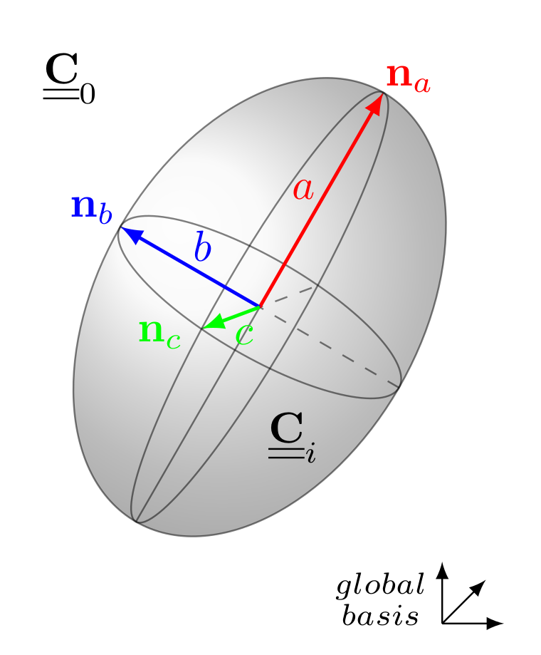
n_a=tm.TVector3D([0.,0.,1.])
n_b=tm.TVector3D([0.,1.,0.])
a=10.
b=1.
c=3.
P2=hm.computeHillTensor(young,nu,n_a,a,n_b,b,c)Note that the above functions have slightly different names from the
C++ version: computeHillPolarisationTensor
becomes computeHillTensor. Moreover, as in
C++, it is possible to pass isotropic moduli objects
instead of young and nu:
IM0=tmat.YoungNuModuli(young,nu)
P0 = hm.computeSphereHillTensor(IM0)
P0_axi = hm.computeAxisymmetricalHillTensor(IM0,n_a,e)
P0_ellipsoid = hm.computeHillTensor(IM0,n_a,a,n_b,b,c)
The computation in the anisotropic reference medium is given by:
C0=tm.ST2toST23D(1e9*np.eye(6))
C0[0,2]=0.1e9
C0[2,0]=0.1e9

max_it=14 #optional

P=hm.computeAnisotropicHillTensor(C0,n_a,a,n_b,b,c,max_it)
Note that the integer max_it is related to the number of
iterations in the integration process (see the documentation of the
namespace).
The computation of the strain localisation tensors are given by:
young=1e9
nu=0.2
young_i=100e9
nu_i=0.3

# Spherical inclusion
A_S=hm.computeSphereLocalisationTensor(young,nu,young_i,nu_i)

# Axisymmetric ellipsoidal inclusion (or spheroid)
e=20.
n=tm.TVector3D([0.,0.,1.])
A_AE=hm.computeAxisymmetricalLocalisationTensor(young,nu,young_i,nu_i,n,e)

# General ellipsoidal inclusion
a=10.
b=1.
c=3.
n_a=tm.TVector3D([0.,0.,1.])
n_b=tm.TVector3D([0.,1.,0.])

A_GE=hm.computeLocalisationTensor(young,nu,young_i,nu_i,n_a,a,n_b,b,c)
Some isotropic moduli can also be passed for the elasticities, as follows:
IM0=tmat.YoungNuModuli(young,nu)
IMi=tmat.YoungNuModuli(young_i,nu_i)
A0 = hm.computeSphereLocalisationTensor(IM0,IMi)
A0_axi = hm.computeAxisymmetricalLocalisationTensor(IM0,IMi,n_a,e)
A0_ellipsoid = hm.computeLocalisationTensor(IM0,IMi,n_a,a,n_b,b,c)
Note that if the elasticity of the inclusion is not isotropic, an
anisotropic elasticity C_i can be provided, assuming that
this elasticiy is expressed in the same basis as the one defined by
n_a,n_b (the local basis of the inclusion):
A_aniso = hm.computeLocalisationTensor(IM0,C_i,n_a,a,n_b,b,c)The case of an anisotropic reference medium is detailed below:
# Anisotropic matrix
max_it=12 #optional
C0_glob=tm.ST2toST23D(1e9*np.eye(6)) # C0_glob is defined in the basis in which the localisation tensor is returned
C0_glob[0,2]=0.1e9
C0_glob[2,0]=0.1e9

Ci_loc=tm.ST2toST23D(1e9*np.eye(6)) # Ci_loc is defined in the basis defined by 'n_a' and 'n_b'

A_AN=hm.computeAnisotropicLocalisationTensor(C0_glob,Ci_loc,n_a,a,n_b,b,c,max_it)
Note that in this case, the elasticity of the inclusion is always
passed as a ST2toST2 object C_i_loc. Moreover,
if this elasticity is not isotropic, C_i_loc is expressed
in the same basis as the one defined by n_a,n_b (the local
basis of the inclusion, see the documentation of the
namespace).
The following schemes are available for biphasic media with 2 isotropic phases:
Here are some examples of computation for the spherical inclusions:
young=1e9
nu=0.2
young_i=100e9
nu_i=0.3
f=0.2
IM=tmat.YoungNuModuli(young,nu)
IMi=tmat.YoungNuModuli(young_i,nu_i)

# Spherical inclusions
EnuDS=hm.computeSphereDiluteScheme(young,nu,f,young_i,nu_i)
EnuMT=hm.computeSphereMoriTanakaScheme(young,nu,f,young_i,nu_i)
KGDS_IM=hm.computeSphereDiluteScheme(IM,f,IMi)
KGMT_IM=hm.computeSphereMoriTanakaScheme(IM,f,IMi)
print(EnuDS.young,EnuDS.nu,KGDS_IM.kappa,KGDS_IM.mu)
print(EnuMT.young,EnuMT.nu,KGMT_IM.kappa,KGMT_IM.mu)
And we can also consider distribution of ellipsoidal inclusions, with three kind of distributions of orientations.
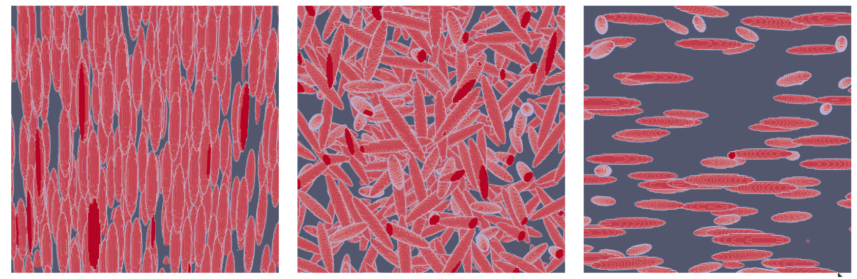
Hence, here are the examples to compute the homogenized properties:
# Ellipsoidal inclusions
a=10.
b=1.
c=3.
n_a=tm.TVector3D([0.,0.,1.])
n_b=tm.TVector3D([0.,1.,0.])

## Isotropic distribution of orientations
KG_I_DS=hm.computeIsotropicDiluteScheme(IM,f,IMi,a,b,c)
KG_I_MT=hm.computeIsotropicMoriTanakaScheme(IM,f,IMi,a,b,c)

D=hm.Distribution(n_a,a,n_b,b,c)
C_I_PCW=hm.computeIsotropicPCWScheme(IM,f,IMi,a,b,c,D)

print(KG_I_DS.kappa,KG_I_DS.mu)
print(KG_I_MT.kappa,KG_I_MT.mu)
print(C_I_PCW)

## Ellipsoids which turn around their axis 'a'
C_TI_DS=hm.computeTransverseIsotropicDiluteScheme(IM,f,IMi,n_a,a,b,c)
C_TI_MT=hm.computeTransverseIsotropicMoriTanakaScheme(IM,f,IMi,n_a,a,b,c)
C_TI_PCW=hm.computeTransverseIsotropicPCWScheme(IM,f,IMi,n_a,a,b,c,D)
print(C_TI_DS)
print(C_TI_MT)
print(C_TI_PCW)

## Oriented ellipsoids
C_O_DS=hm.computeOrientedDiluteScheme(IM,f,IMi,n_a,a,n_b,b,c)
C_O_MT=hm.computeOrientedMoriTanakaScheme(IM,f,IMi,n_a,a,n_b,b,c)
C_O_PCW=hm.computeOrientedPCWScheme(IM,f,IMi,n_a,a,n_b,b,c,D)
print(C_O_DS)
print(C_O_MT)
print(C_O_PCW)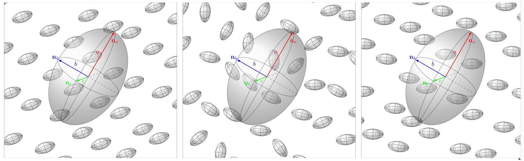
In Ponte-Castaneda and Willis scheme (PCW), there is a difference
between the ellipsoid which defines the distribution of the inclusions,
and the ellipsoid which defines the shape of the inclusions (in the
image above, we represent the distribution D of inclusions
by a big ellipsoid, with colored axes). A bigger axis for D
means that along this axis, the distribution of inclusions is more
diluted. A short axis means that, on the contrary, the distribution is
denser along this axis. The object D is defined above at
line 12.
The available bounds are:
Here are some examples of computation:
f0=0.2
f1=0.5
f2=0.3
C0=tm.ST2toST23D(np.eye(6))
C1=tm.ST2toST23D(2*np.eye(6))
C2=tm.ST2toST23D(5*np.eye(6))

C0_2d=tm.ST2toST22D(np.eye(4))
C1_2d=tm.ST2toST22D(2*np.eye(4))
C2_2d=tm.ST2toST22D(5*np.eye(4))

# Voigt and Reuss bounds
CV_3D=hm.computeVoigtStiffness3D([f0,f1,f2],[C0,C1,C2])
CV_2D=hm.computeVoigtStiffness2D([f0,f1,f2],[C0_2d,C1_2d,C2_2d])
CR_3D=hm.computeReussStiffness3D([f0,f1,f2],[C0,C1,C2])
CR_2D=hm.computeReussStiffness2D([f0,f1,f2],[C0_2d,C1_2d,C2_2d])

print(CR_3D,CV_3D)
print(CR_2D,CV_2D)

# Hashin-Shtrikman bounds
K0=1/3
G0=1/2
K1=2/3
G1=1
K2=5/3
G2=5/2
KG_HS_3D=hm.computeIsotropicHashinShtrikmanBounds3D([f0,f1,f2],[K0,K1,K2],[G0,G1,G2])
KG_HS_2D=hm.computeIsotropicHashinShtrikmanBounds2D([f0,f1,f2],[K0,K1,K2],[G0,G1,G2])

K_LB_3D=KG_HS_3D[0][0]
G_LB_3D=KG_HS_3D[0][1]
K_UB_3D=KG_HS_3D[1][0]
G_UB_3D=KG_HS_3D[1][1]

print(K_LB_3D,G_LB_3D)
print(K_UB_3D,G_UB_3D)

K_LB_2D=KG_HS_2D[0][0]
G_LB_2D=KG_HS_2D[0][1]
K_UB_2D=KG_HS_2D[1][0]
G_UB_2D=KG_HS_2D[1][1]

print(K_LB_2D,G_LB_2D)
print(K_UB_2D,G_UB_2D)
Note that Voigt and Reuss bounds work on ST2toST2
objects, whereas Hashin-Shtrikman bounds work on bulk and shear moduli.
The number of phases is arbitrary.
ParticulateMicrostructureSome objects are defined that mirror the objects defined in the
namespace tfel::material::homogenization::elasticity for
the construction and homogenization of general microstructures. The
reader may want to consult this documentation here.
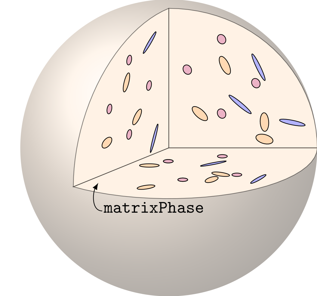
The ParticulateMicrostructure object is defined and can
be instantiated in various ways:
IM0=tmat.KGModuli(1e7,1e7)
micro_1=hm.ParticulateMicrostructure(IM0)

C0=tm.ST2toST23D(1e7*np.eye(6))
micro_2=hm.ParticulateMicrostructure(C0)

micro_3=hm.ParticulateMicrostructure(micro_2)
where C0 and IM0 correspond to the
elasticity of the matrix phase. The
ParticulateMicrostructure has no public attribute. However,
it has some methods that return the value of the private attributes:
print(micro_1.getNumberOfPhases())
print(micro_1.getMatrixFraction())
print(micro_1.getMatrixElasticity())
print(micro_1.isIsotropicMatrix())
Note that last line returns True if micro_1
was instantiated with objects like KGModuli,
YoungNuModuli, LambdaMuModuli, and
False when instantiated with a ST2toST2 (like
micro_2 above).
We can add a distribution of inclusions if we first instantiate such a distribution. We must instantiate an inclusion first:
a=10
b=2
c=3
sph=hm.Sphere()
spheroid=hm.Spheroid(a,b)
ellipso=hm.Ellipsoid(a,b,c)
print(spheroid.axis_length(),spheroid.transverse_length())
print(ellipso.semi_lengths)
We can now instantiate a distribution of inclusions in various ways:
IMi=tmat.KGModuli(1e9,1e9)
f=0.1
sph_dist=hm.SphereDistribution(sph,f,IMi)
ellipsoid_dist_iso=hm.IsotropicDistribution(ellipso,f,IMi)

n_a=tm.TVector3D([0.,0.,1.])
n_b=tm.TVector3D([0.,1.,0.])
ellipsoid_dist_O=hm.OrientedDistribution(ellipso,f,IMi,n_a,n_b)
Ci=tm.ST2toST23D(1e9*np.eye(6))
Ci[0,1]=1e8
Ci[1,0]=1e8
ellipsoid_dist_O_2=hm.OrientedDistribution(ellipso,f,Ci,n_a,n_b)
The TransverseDistribution is a special case which
requires to precise which axis of the ellipsoid (or spheroid) will
remain fixed when the two other axes rotate:
index=0
ellipsoid_dist_TI=hm.TransverseIsotropicDistribution(ellipso,f,IMi,n_a,index)
The index can be 0,1 or 2. For a spheroid, giving 2 for
the index is the same as giving 1, because
these 2 axes have the same length.
Note that the OrientedDistribution can be instantiated
with a ST2toST2 object, here Ci. It is also
possible for a SphereDistribution. It can be useful for
considering anisotropic inclusions. However, the basis in which
Ci is defined is the local basis for the
OrientedDistribution, that is, the basis defined by
n_a and n_b passed as arguments. For a
SphereDistribution, it is the global basis.
Another type of distribution can be defined: the
UserDefinedDistributionOfSpheroids. This is a distribution
of spheroids defined with two orientation tensors, that incorporate
microstructural information about the orientations of the spheroids (see
here
for the definition of orientation tensors). This kind of distribution
can be constructed with Spheroid objects only. This is done
as follows:
spheroid=Spheroid(10,1)
KGi=KGModuli(300,200)
A2=Stensor3D([1.,1.,1.,0.,0.,0.])
tenseur=np.zeros((6,6))
tenseur[0,0]=0.1
A4=ST2toST23D(np.eye(6)+tenseur)
distrib=UserDefinedDistributionOfSpheroids(spheroid,frac,KGi,A2,A4)
Above, the tensor A2 is the second-order orientation
tensor, taken equal to \(\frac13\mathbf
1\), and A4 is the fourth-order orientation tensor,
which is, here, particular.
We can now add these distributions to the microstructure:
micro_1.addInclusionPhase(sph_dist)
print(micro_1.getNumberOfPhases())
print(micro_1.getMatrixFraction())

micro_1.addInclusionPhase(ellipsoid_dist_iso)
print(micro_1.getNumberOfPhases())
print(micro_1.getMatrixFraction())
or remove them:
micro_1.removeInclusionPhase(0)
print(micro_1.getNumberOfPhases())
print(micro_1.getMatrixFraction())
At this stage, we have added the distribution of spheres
sph_dist, and added the isotropic distribution of
ellipsoids ellipsoid_dist_iso. Afterthat, we have removed
the first inclusion distribution (number 0), which is the
distribution of spheres. Hence, only one
InclusionDistribution object remains in the microstructure.
We can get this distribution by doing:
ell_dist=micro_1.getInclusionPhase(0)This distribution of ellipsoids was instantiated before with a
Ellipsoid object, a fraction, and an isotropic elastic
modulus (see above ellipsoid_dist_iso) In fact, the
distribution has three attributes:
print(ell_dist.inclusion)
print(ell_dist.fraction)
print(ell_dist.getElasticityOfPhase())
like the other types of distributions of inclusions
(SphereDistribution,
TransverseIsotropicDistribution and
OrientedDistribution). All these distributions have also
two methods. The first just states if the distribution was instantiated
with isotropic elastic moduli or with a ST2toST2 object.
Here, it was instantiated with a KGModuli, so that it is
considered isotropic. Hence,
print(ell_dist.isIsotropic())returns True.
The second method of the distribution allows to compute the mean strain localisation (or concentration) tensor in the inclusions when they are embedded in a matrix:
Ai=ell_dist.computeMeanLocalisator(IM0)
print(Ai)
Note that in the latter case, passing C0, a
ST2toST2 object as an argument of the method will return an
error, because it will be considered that the matrix is not isotropic,
so that computing a average localisator of a distribution of ellipsoids
in an anisotropic matrix is impossible (too complicated). However, it
can be done for other kinds of distributions, like sphere distributions
or distributions of oriented inclusions:
A1=sph_dist.computeMeanLocalisator(C0,10)
A2=ellipsoid_dist_O.computeMeanLocalisator(C0,10)
print(A1,A2)
Here, the integer 10 is the number of subdivisions in
the integration process in the computation of the Hill tensor relative
to the inclusions. It is 12 by default.
The last method of the ParticulateMicrostructure object
allows to change the elasticity of the matrix phase:
micro_1.changeElasticityOfMatrixPhase(C0)
print(micro_1.getMatrixElasticity())
print(micro_1.isIsotropicMatrix())
Here we see that the matrix is no more isotropic because it was
replaced via a ST2toST2 object.
Now, let us do homogenization !
Three schemes are currently available:
Let us consider the previous ParticulateMicrostructure
object micro_1. We already have seen that computing some
average localisators in an anisotropic matrix was not possible for
non-oriented anisotropic inclusions like ellipsoids. Hence, we here
recover the isotropic matrix by doing
micro_1.changeElasticityOfMatrixPhase(IM0)
print(micro_1.isIsotropicMatrix())
Afterwards,
hmDS=hm.computeDiluteScheme(micro_1)
hmMT=hm.computeMoriTanakaScheme(micro_1)
hmSC=hm.computeSelfConsistentScheme(micro_1,1e-6,True)
print("DS: ",hmDS.homogenized_stiffness)
print("MT: ",hmMT.homogenized_stiffness)
print("SC: ",hmSC.homogenized_stiffness)
We note that computeSelfConsistentScheme not only takes
the microstructure as an argument, but also takes one real
(1e-6) as a parameter, which pilots the precision of the
result. Indeed, at each iteration of the self-consistent iterative
algorithm, the function computes the relative difference between the new
and the old homogenized stiffness. This relative difference must be
smaller than the tolerance given as a parameter. Moreover, the
bool parameter (True) precises if the
computation considers an isotropic matrix when computing the Hill
tensors relative to the inclusions, at each iteration of the algorithm.
Indeed, the homogenized stiffness may be non isotropic, so that the user
can make the choice of isotropizing this homogenized stiffness at each
iteration. Otherwise, he can put False, so that a numerical
integration (resulting in a slower computation) will be performed to
compute the Hill tensors. Moreover, an integer parameter can be added
after the boolean, that indicates the number of subdivisions in the
numerical integration. This value is 12 by default:
micro_2.addInclusionPhase(ellipsoid_dist_O)
hmSC_iso=hm.computeSelfConsistentScheme(micro_2,10,True)
hmSC_aniso=hm.computeSelfConsistentScheme(micro_2,10,False,10)
print("SC iso: ",hmSC_iso.homogenized_stiffness)
print("SC aniso: ",hmSC_aniso.homogenized_stiffness)
For the oter schemes, the isotropic character of the matrix when
computing the strain localisators will depend on what returns
micro_1.isIsotropicMatrix(). Hence, it is important to
initialized the matrix or the microstructure with the appropriate
elastic moduli. If isotropic, it will works in all case, whereas if not
isotropic, it will fail depending on the distributions that are present
in the microstructure. Moreover, if anisotropic, another parameter can
be passed to specify the number of subdivisions in the numerical
integration (this value is 12 by default):
micro_1.changeElasticityOfMatrixPhase(C0)
micro_1.removeInclusionPhase(0)
micro_1.addInclusionPhase(ellipsoid_dist_O)
hmDS_aniso=hm.computeDiluteScheme(micro_1,10)
hmMT_aniso=hm.computeMoriTanakaScheme(micro_1,10)
We can also recover the strain localisation tensors:
A_i_DS=hmDS.mean_strain_localisation_tensors
print("A_0_DS: ",A_i_DS[0],"A_1_DS: ",A_i_DS[1])
We can also add a polarization on each phase:
micro_1.changeElasticityOfMatrixPhase(IM0)
pola=[tm.Stensor3D(6*[0.]),tm.Stensor3D([1.e8,1e8,1e8,0.,0.,0.])]
hmDS_pola=hm.computeDiluteScheme(micro_1,polarisations=pola)
(note that here we must precise the name of the optional argument). And we can recover the effective polarization:
P_eff_DS=hmDS_pola.effective_polarisation
print("P_eff_DS: ",P_eff_DS)
In fact, the functions computeDiluteScheme,
computeMoriTanakaScheme
computeSelfConsistentScheme… return an object
HomogenizationScheme which possesses the attributes
homogenized_stiffness,mean_strain_localisation_tensors
and effective_polarisation.