We are pleased to announce that the next MFront User Meeting will be organized by IMSIA (Institute of Mechanical Sciences and Industrial Applications, UMR 9219 CNRS-EDF-CEA-ENSTA).
The User Meeting will be held on October 17 2019 near Paris on the « Plateau of Saclay ». Do not miss this event, which is a great opportunity to communicate with MFront users.
The program of the day is mostly defined (new contributions are still welcomed). Following feedbacks from previous meetings:
We will made a short introduction to MFront on computers on the morning of October 18 (places will be limited, only a few left) before the “Meeting on Computational Mechanics” at EDF Lab Saclay organized for the 30 years of code_aster.
Access to the user meeting is free but, to facilitate the organization of this event, registration is required. Please register at tfel-contact@cea.fr.
While registering, let us know if you would like to present your work and/or if you would like attend to the first part of the meeting and/or to the second part and/or if you would be interested by the introduction on October 18.
MFront code
generator (24/01/2019)Du to Jeremy Bleyer a new tutorial on how to use MFront
with FEniCS in pure python is available: https://comet-fenics.readthedocs.io/en/latest/demo/plasticity_mfront/plasticity_mfront.py.html
This is based on the MGIS
(MFrontGenericInterfaceSupport) python bindings (and not
the FEniCS bindings which are only available in
C++ and currently quite limited), which makes it very easy
to use and extend.
You can now use any small strain behaviours written in
MFront. Extension to finite strain behaviours is underway
and shall be soon available. This development will also help testing the
extension of MFront to generalised behaviours,able to cope
with higher order mechanical theories (Cosserat medium for instance)
and/or multi-physics problems.
TFEL
is available as a spack package (27/11/2018)One easy way to install TFEL under LiNuX
and MacOs is to use the spack package
manager.
The spack package manager is fully described here: https://spack.readthedocs.io/en/latest/index.html
The following instructions will build the latest development versions:
$ git clone --single-branch -b develop https://github.com/spack/spack.git
$ . spack/share/spack/setup-env.sh
$ spack install tfel@master
The TFEL package can then be loaded as follows:
$ spack load tfel@masterOne nifty feature of spack is that you can install
various versions of TFEL in parallel.
This project is meant to ease the integration of MFront in various environments, including homebrew solvers (FE, FFT, etc…). Source code can be found here:
https://github.com/thelfer/MFrontGenericInterfaceSupport.git
The project has a permissive licence for it to be used in both commercial or open-source codes.
Bindings for C are already available. Do not hesitate to
consider developping bindings for other languages, such as
Python, Fortran, Julia,
Java, Matlab, GNU
Octave, Scilab, etc.
We are pleased to announce the fourth MFront User Day that will held at Cadarche on October the 16th of 2018.
This day will give the opportunity for the developers to present the numerous new features of the 3.2 version and for the users to present their works and to make feed-backs.
All the contributions are welcomed, do not hesitate to contact the organizers to present your work.
The agenda and the location will be communicated later.
The event is free and open to all. However, registration is mandatory. Please send the organizers at the following information:
Please register your participation before September 15th 2018 to facilitate the organisation.
TFEL/MFront project on ResearchGate (28/06/2018)TFEL/MFront meets a growing success in the academic
work. A ResearchGate project has been created to accompagny
this rise:
https://www.researchgate.net/project/TFEL-MFront
TFEL/MFront at Centrale Lille
(21/06/2018)On the 21th of May, we had the chance to make a seminar about
TFEL/MFront at [Centrale Lille.
The talk is available here: https://github.com/thelfer/tfel-doc/tree/master/Talks/CentraleLille2018.
TFEL/MFront at the ENSMM (7/06/2018)On the 7th of May, we had the chance to make a seminar about
TFEL/MFront at the ENSMM
(École nationale supérieure de mécanique et des microtechniques)
Besançon in the Departement of Applied Mechanics.
The talk is available here: https://github.com/thelfer/tfel-doc/tree/master/Talks/ENSMM2018.
TFEL/MFront (31/05/2018)In prevision of the forthcoming release of the Alcyone
fuel performance code, TFEL 3.1.2 has been released. This
is mostly a bug fix. Thanks to all the users who reported the issues and
contributed to the enhancement of TFEL/MFront.
A special focus is made on Ticket
#127 that may change the results of badly convergent behaviours
using sub-stepping with the Cast3M and Cyrano
interfaces.
A detailed version of the release notes is available here.
Cast3M 2018 has
been released.
Binary package for Cast3M 2018 and
Windows 64 are now available for download: https://sourceforge.net/projects/tfel/files.
See also the example: http://tfel.sourceforge.net/downloads/windows-install-scripts.tar.bz2.
The test directory contains an example showing how to use this binary
package. Be sure to change the PATH variable to match your
installation directories at the beginning of the
mfront-Cast3M2018.bat and
launch-Cast3M2018.bat files.
The yield surface is combining two surfaces:

This video reproduces the work of Yoon et al (See [2]). in Abaqus/Standard and Abaqus/Explicit. The material is described by Barlat’ Yld2004-18p yield function (See [3]), as described here.

A new paper using MFront has been published in the
Journal of Nuclear Materials ([4]). See https://doi.org/10.1016/j.jnucmat.2018.01.064 for the
online version.
")
Giacomo Torelli (The University of Cambridge), Parthasarathi Mandal (The University of Manchester) and Martin Gillie (The University of Warwick) developed a new constitutive laws describing the Load-Induced-Thermal-Strain (LITS) which captures the experimentally demonstrated behaviour of concrete in the case of heating under multiaxial mechanical load, for temperatures up to \(500\mbox^{\circ{}}C\).
In contrast to the models available in the literature, this new behaviour takes into account the observed dependency of LITS on stress confinement. Such a dependency is introduced through a confinement coefficient which makes LITS directly proportional to the confinement of the stress state.
Details of theoretical and numerical implementation can be found in [5].
The implementation of the behaviour is available in the
MFrontGallery here.
TFEL/MFront (7/03/2017)In prevision of the 14.2 release of Code_Aster and 2018
release of Salome-Meca, TFEL 3.1.1 has been
released. This is mostly a bug fix version with a few enhancements.
A detailed version of the release notes is available here.
Within the framework of the theory of representation, generalizations to orthotropic conditions of the invariants of the deviatoric stress have been proposed by Cazacu and Barlat (see [6]):
Those invariants may be used to generalize isotropic yield criteria based on \(J_{2}\) and \(J_{3}\) invariants to orthotropy.
The following functions
\(J_{2}^{0}\), \(J_{3}^{0}\) and their first and second derivatives with respect to the stress tensor \(\underline{\sigma}\) can be computed by the following functions:
computesJ2O, computesJ2ODerivative and
computesJ2OSecondDerivative.computesJ3O, computesJ3ODerivative and
computesJ3OSecondDerivative.Those functions take the stress tensor as first argument and each
orthotropic coefficients. Each of those functions has an overload taking
the stress tensor as its firs arguments and a tiny vector
(tfel::math::tvector) containing the orthotropic
coefficients.
Let \(\underline{\sigma}\) be a stress tensor. Its deviatoric part \(\underline{s}\) is:
\[ \underline{s}=\underline{\sigma}-{{\displaystyle \frac{\displaystyle 1}{\displaystyle 3}}}\,{\mathrm{tr}{\left(\underline{\sigma}\right)}}\,\underline{I} ={\left(\underline{\underline{\mathbf{I}}}-{{\displaystyle \frac{\displaystyle 1}{\displaystyle 3}}}\,\underline{I}\,\otimes\,\underline{I}\right)}\,\colon\,\underline{\sigma} \]
The deviator of a tensor can be computed using the
deviator function.
As it is a second order tensor, the stress deviator tensor also has a set of invariants, which can be obtained using the same procedure used to calculate the invariants of the stress tensor. It can be shown that the principal directions of the stress deviator tensor \(s_{ij}\) are the same as the principal directions of the stress tensor \(\sigma_{ij}\). Thus, the characteristic equation is
\[ \left| s_{ij}- \lambda\delta_{ij} \right| = -\lambda^3+J_1\lambda^2-J_2\lambda+J_3=0, \]
where \(J_1\), \(J_2\) and \(J_3\) are the first, second, and third deviatoric stress invariants, respectively. Their values are the same (invariant) regardless of the orientation of the coordinate system chosen. These deviatoric stress invariants can be expressed as a function of the components of \(s_{ij}\) or its principal values \(s_1\), \(s_2\), and \(s_3\), or alternatively, as a function of \(\sigma_{ij}\) or its principal values \(\sigma_1\), \(\sigma_2\), and \(\sigma_3\). Thus,
\[ \begin{aligned} J_1 &= s_{kk}=0,\, \\ J_2 &= \textstyle{\frac{1}{2}}s_{ij}s_{ji} = {{\displaystyle \frac{\displaystyle 1}{\displaystyle 2}}}{\mathrm{tr}{\left(\underline{s}^2\right)}}\\ &= {{\displaystyle \frac{\displaystyle 1}{\displaystyle 2}}}(s_1^2 + s_2^2 + s_3^2) \\ &= {{\displaystyle \frac{\displaystyle 1}{\displaystyle 6}}}\left[(\sigma_{11} - \sigma_{22})^2 + (\sigma_{22} - \sigma_{33})^2 + (\sigma_{33} - \sigma_{11})^2 \right ] + \sigma_{12}^2 + \sigma_{23}^2 + \sigma_{31}^2 \\ &= {{\displaystyle \frac{\displaystyle 1}{\displaystyle 6}}}\left[(\sigma_1 - \sigma_2)^2 + (\sigma_2 - \sigma_3)^2 + (\sigma_3 - \sigma_1)^2 \right ] \\ &= {{\displaystyle \frac{\displaystyle 1}{\displaystyle 3}}}I_1^2-I_2 = \frac{1}{2}\left[{\mathrm{tr}{\left(\underline{\sigma}^2\right)}} - \frac{1}{3}{\mathrm{tr}{\left(\underline{\sigma}\right)}}^2\right],\,\\ J_3 &= \det(s_{ij}) \\ &= {{\displaystyle \frac{\displaystyle 1}{\displaystyle 3}}}s_{ij}s_{jk}s_{ki} = {{\displaystyle \frac{\displaystyle 1}{\displaystyle 3}}} {\mathrm{tr}{\left(\underline{s}^3\right)}}\\ &= {{\displaystyle \frac{\displaystyle 1}{\displaystyle 3}}}(s_1^3 + s_2^3 + s_3^3) \\ &= s_1s_2s_3 \\ &= {{\displaystyle \frac{\displaystyle 2}{\displaystyle 27}}}I_1^3 - {{\displaystyle \frac{\displaystyle 1}{\displaystyle 3}}}I_1 I_2 + I_3 = {{\displaystyle \frac{\displaystyle 1}{\displaystyle 3}}}\left[{\mathrm{tr}{\left(\underline{\sigma}^3\right)}} - {\mathrm{tr}{\left(\underline{\sigma}^2\right)}}{\mathrm{tr}{\left(\underline{\sigma}\right)}} +{{\displaystyle \frac{\displaystyle 2}{\displaystyle 9}}}{\mathrm{tr}{\left(\underline{\sigma}\right)}}^3\right]. \end{aligned} \]
where \(I_{1}\), \(I_{2}\) and \(I_{3}\) are the invariants of \(\underline{\sigma}\).
\(J_{2}\) and \(J_{3}\) are building blocks for many isotropic yield critera. Classically, \(J_{2}\) is directly related to the von Mises stress \(\sigma_{\mathrm{eq}}\):
\[ \sigma_{\mathrm{eq}}=\sqrt{{{\displaystyle \frac{\displaystyle 3}{\displaystyle 2}}}\,\underline{s}\,\colon\,\underline{s}}=\sqrt{3\,J_{2}} \]
The first and second derivatives of \(J_{2}\) with respect to \(\sigma\) can be trivially implemented, as follows:
constexpr const auto id  = stensor<N,real>::Id();
constexpr const auto id4 = st2tost2<N,real>::Id();
// first derivative of J2
const auto dJ2  = deviator(sig);
// second derivative of J2
const auto d2J2 = eval(id4-(id^id)/3);
In comparison, the computation of the first and second derivatives of
\(J_{3}\) with respect to \(\sigma\) are more cumbersome. In previous
versions TFEL, one had to write:
constexpr const auto id = stensor<N,real>::Id();
constexpr const auto id4 = st2tost2<N,real>::Id();
const auto I1   = trace(sig);
const auto I2   = (I1*I1-trace(square(sig)))/2;
const auto dI2  = I1*id-sig;
const auto dI3  = computeDeterminantDerivative(sig);
const auto d2I2 = (id^id)-id4;
const auto d2I3 = computeDeterminantSecondDerivative(sig);
// first derivative of J3
const auto dJ3  = eval((2*I1*I1/9)*id-(I2*id+I1*dI2)/3+dI3);
// second derivative of J3
const auto d2J3 = eval((4*I1/9)*(id^id)-((id^dI2)+(dI2^id)+i1*d2I2)/3+d2I3);
More efficient implementations are now available using the
computeDeviatorDeterminantDerivative and
computeDeviatorDeterminantSecondDerivative functions:
// first derivative of J3
const auto dJ3  = computeDeviatorDeterminantDerivative(sig);
// second derivative of J3
const auto d2J3 = computeDeviatorDeterminantSecondDerivative(sig);doxygen
documentation (4/01/2018)Further documentation for advanced users has been published: the
internal code documentation of the project, as generated by doxygen, is now available
online:
http://tfel.sourceforge.net/doxygen/index.html
The theme has been adapted from:
https://github.com/Velron/doxygen-bootstrapped
TFEL/MFront (15/12/2017)Versions 3.1 and 3.0.3 of TFEL, MFront and
MTest has been released on the 15th December, 2017.
A detailed version of the release notes is available here.
From a user point of view, TFEL 3.1 brings many important features:
MFront that will be updated as TFEL and MFront evolve. In
each case, the integration algorithm is fully described. The gallery
currently contains \(17\) entries
covering finite strain elasticity, finite strain viscoplasticity,
damage, plasticity and viscoplasticity. The gallery. Those
implementations are also gathered in a cmake projects
called MFrontGallery which can be cloned on github: https://github.com/thelfer/MFrontGalleryTFEL/NUMODIS library which
provides many functionalities associated with single crystal description
coming from the NUMODIS
project. Those functionalities are available in MFront
through many new keywords that simplify to a great extent the way small
and finite strain single crystal behaviours can be written. See the
following page for a detailled description: http://tfel.sourceforge.net/singlecrystal.htmlDDIF2 behaviour is used in CEA fuel performances
codes to describe cracking of the nuclear fuel. The DDIF2
brick allows this model to be easily coupled to the viscplastic
behaviour of the fuel material and can be used as easily as the
StandardElasticity brick. See this page for details: http://tfel.sourceforge.net/ddif2.htmlTFEL/Math. It is now much safer to use the
-ffast-math option in gcc and
clang which can drastically increase the efficiency of the
generated code. This option is automatically added when using the
--obuild=level2 option of mfront. See the
release notes for details.MTest.cmake
generator, using mfront on windows with the
Microsoft compilers is easy and closely follows the
existing practices on other operating systems.TFEL/MFront can now be installed in
parallel. See http://tfel.sourceforge.net/install.html for
details.Two new interfaces have been introduced in MFront:
CalculiX solver. Here native
is used to distinguish this interface from the
Abaqus/Standard interface which can also be used within
CalculiX. This interface can be used with
CalculiX 2.13.ANSYS APDL solver.
The latter is still experimental.@NumericallyComputedJacobianBlocks keywordComputing the jacobian of the implicit system is the most difficult part of implementing a behaviour. Computing the jacobian by finite difference is interesting but significantly decreases the performances of the behaviour and can be (very) sensitive to the choice of the numerical perturbation.
The @NumericallyComputedJacobianBlocks keyword is used
select a list of jacobian blocks that have to be computed numerically.
This is more efficient than computing the whole jacobian numerically.
Combined with the ability to compare the jacobian to a numerical
approximation, the user now has the ability to build the jacobian
incrementally, block by block and checks at each steps that their
analytical expressions are correct.
Portability is a convincing sign of software quality and maintainability:
C or C++
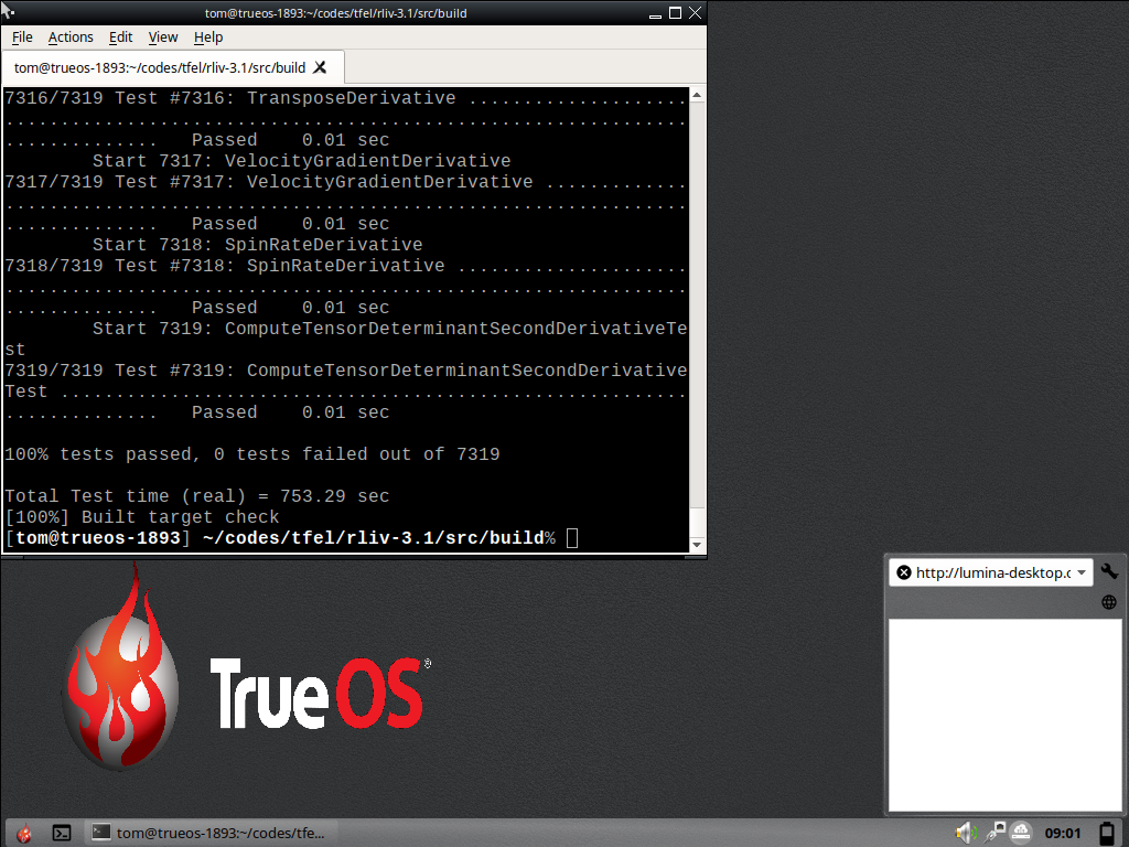
libraries.TFEL has been tested successfully on a various flavours
of LinuX and BSD systems (including
FreeBSD and OpenBSD). The first ones are
mostly build on gcc, libstdc++ and the
glibc. The second ones are build on clang and
libc++.
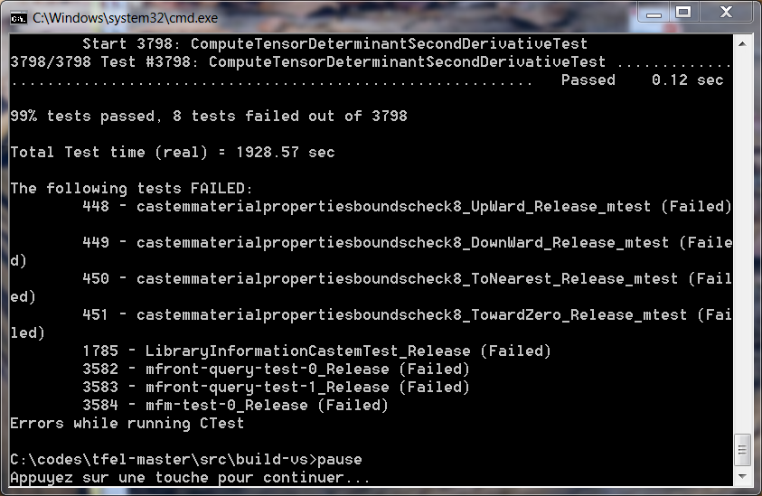
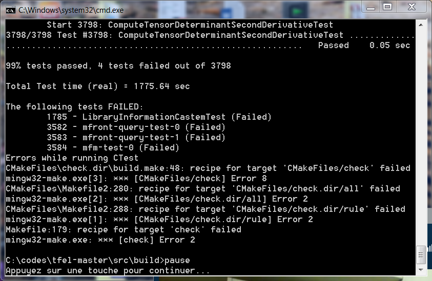
TFEL can be build on Windows in a wide
variety of configurations and compilers:
Visual Studio (2015
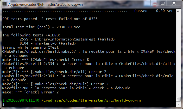
and 2017) or MingGW compilers.TFEL can be build in the Cygwin
environment.TFEL have reported to build successfully in the
Windows Subsystem for LinuX (WSL)
environment.
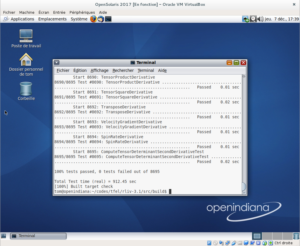
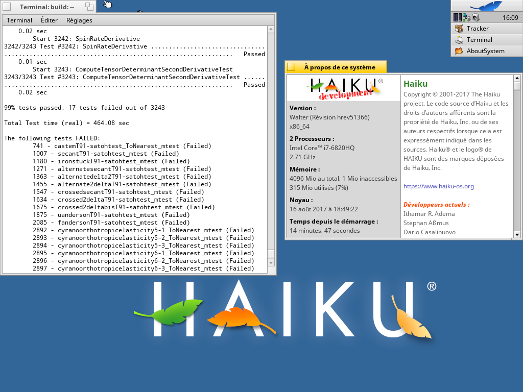
Although not officially supported, more exotic systems, such as
OpenSolaris and Haiku, have also been tested
successfully. The Minix operating systems provides a
pre-release of clang 3.4 that fails to compile
TFEL.
Version 3.1 has been tested using the following compilers:
gcc on various
POSIX systems: versions 4.7, 4.8, 4.9, 5.1, 5.2, 6.1, 6.2,
7.1, 7.2clang on various
POSIX systems: versions 3.5, 3.6, 3.7, 3.8, 3.9, 4.0,
5.0intel.
The only tested version is the 2018 version on LinuX. Intel compilers
15 and 16 are known not to work due to a bug in the EDG front-end that can’t parse a syntax
mandatory for the expression template engine. The same bug affects the
Blitz++ library
(see http://dsec.pku.edu.cn/~mendl/blitz/manual/blitz11.html).
Version 2017 shall work but were not tested.Visual Studio The
only supported versions are the 2015 and 2017 versions. Previous
versions do not provide a suitable C++11 support.PGI compiler (NVIDIA): version 17.10 on
LinuXMinGW has been tested successfully in a wide variety of
configurations/versions, including the version delivered with
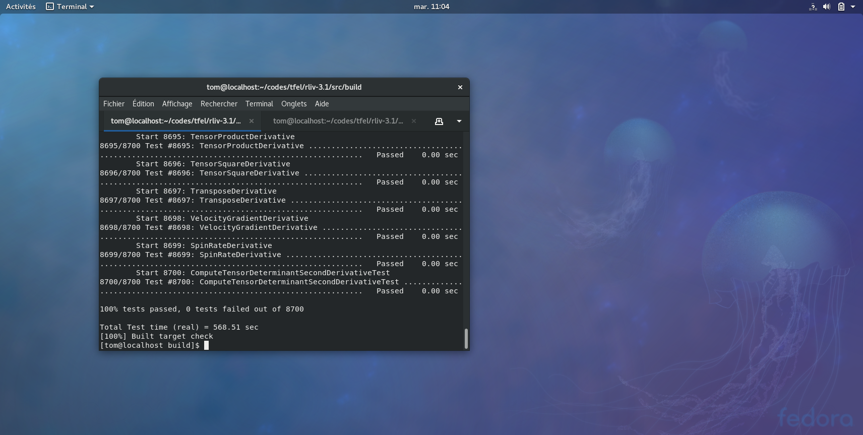
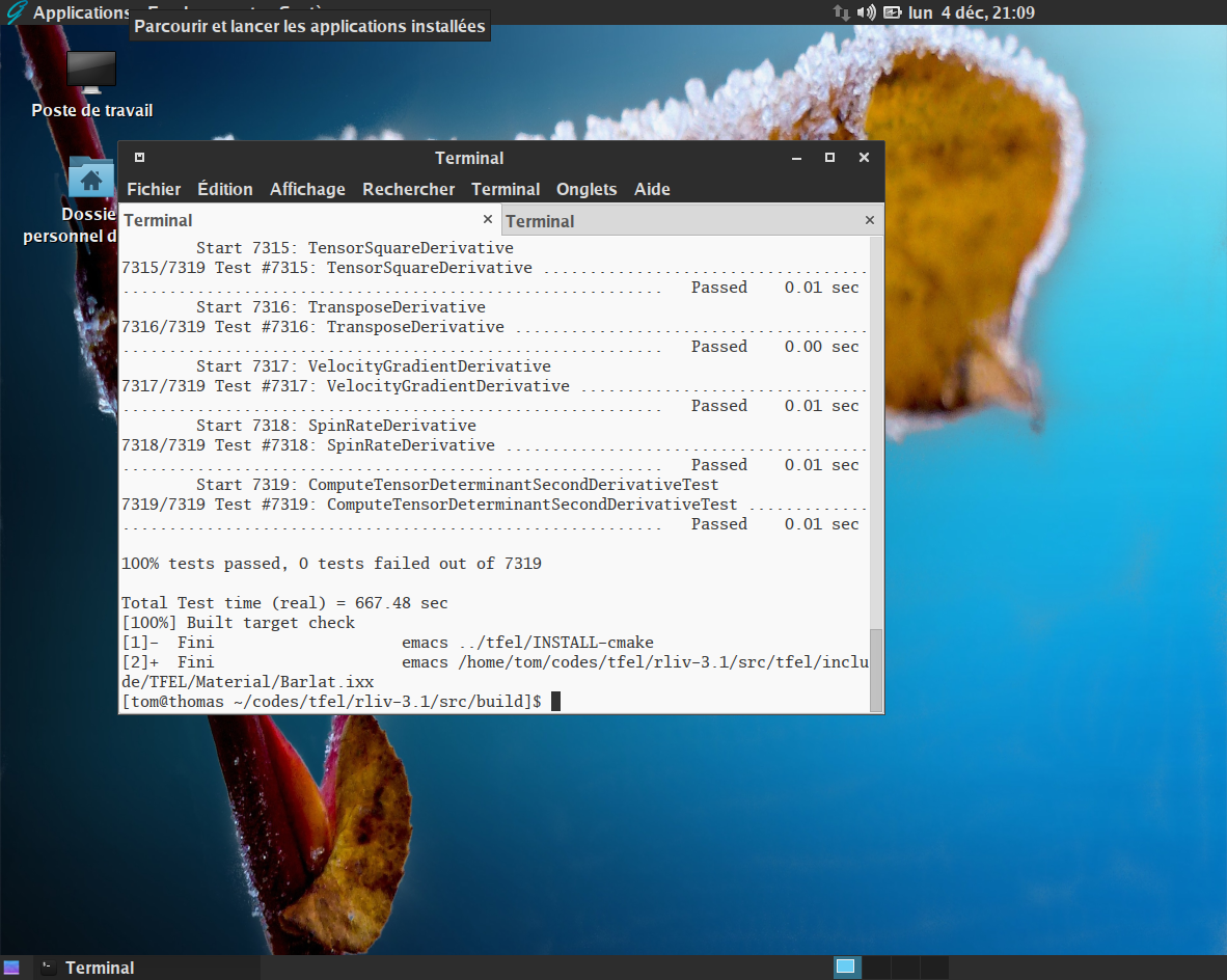
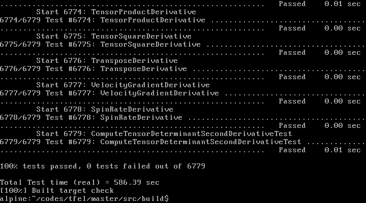
Cast3M 2017.| Compiler and options | Success ratio | Test time |
|---|---|---|
gcc 4.9.2 |
100% tests passed | 681.19 sec |
gcc 4.9.2+fast-math |
100% tests passed | 572.48 sec |
clang 3.5 |
100% tests passed | 662.50 sec |
clang 3.5+libstcxx |
99% tests passed | 572.18 sec |
clang 5.0 |
100% tests passed | 662.50 sec |
icpc 2018 |
100% tests passed | 511.08 sec |
PGI 17.10 |
99% tests passed | 662.61 sec |
Concerning the PGI compilers, performances may be
affected by the fact that this compiler generates huge shared libraries
(three to ten times larger than other compilers).
This is mainly a bug fix version of the 3.0 series.
Detailed release notes are available here. There are no known
regressions.
 and the von Mises criterion in plane stress")
The Green yield criterion is based on the definition of an equivalent stress \(\sigma_{\mathrm{eq}}\) defined as follows: \[ \sigma_{\mathrm{eq}}=\sqrt{{{\displaystyle \frac{\displaystyle 3}{\displaystyle 2}}}\,C\,\underline{s}\,\colon\,\underline{s}+F\,{\mathrm{tr}{\left(\underline{\sigma}\right)}}^{2}} \] where \(\underline{s}\) is the deviatoric stress tensor: \[ \underline{s}=\underline{\sigma}-{{\displaystyle \frac{\displaystyle 1}{\displaystyle 3}}}\,{\mathrm{tr}{\left(\underline{\sigma}\right)}}\,\underline{I} \]
A new entry in the gallery shows how to build a perfect plastic behaviour based on this equivalent stress. The implementation is available here: https://github.com/thelfer/MFrontGallery/blob/master/generic-behaviours/plasticity/GreenPerfectPlasticity.mfront
Functions to compute the Barlat equivalent stress and its first and
second derivatives are now available in TFEL/Material.
The Barlat equivalent stress is defined as follows (See [3]): \[ \sigma_{\mathrm{eq}}^{B}= \sqrt[a]{ \frac{1}{4}\left( \sum_{i=0}^{3} \sum_{j=0}^{3} {\left|s'_{i}-s''_{j}\right|}^{a} \right) } \]
where \(s'_{i}\) and \(s''_{i}\) are the eigenvalues of two transformed stresses \(\underline{s}'\) and \(\underline{s}''\) by two linear transformation \(\underline{\underline{\mathbf{L}}}'\) and \(\underline{\underline{\mathbf{L}}}''\): \[ \left\{ \begin{aligned} \underline{s}' &= \underline{\underline{\mathbf{L'}}} \,\colon\,\underline{\sigma}\\ \underline{s}'' &= \underline{\underline{\mathbf{L''}}}\,\colon\,\underline{\sigma}\\ \end{aligned} \right. \]
The linear transformations \(\underline{\underline{\mathbf{L}}}'\) and \(\underline{\underline{\mathbf{L}}}''\) are defined by \(9\) coefficients (each) which describe the material orthotropy. There are defined through auxiliary linear transformations \(\underline{\underline{\mathbf{C}}}'\) and \(\underline{\underline{\mathbf{C}}}''\) as follows: \[ \begin{aligned} \underline{\underline{\mathbf{L}}}' &=\underline{\underline{\mathbf{C}}}'\,\colon\,\underline{\underline{\mathbf{M}}} \\ \underline{\underline{\mathbf{L}}}''&=\underline{\underline{\mathbf{C}}}''\,\colon\,\underline{\underline{\mathbf{M}}} \end{aligned} \] where \(\underline{\underline{\mathbf{M}}}\) is the transformation of the stress to its deviator: \[ \underline{\underline{\mathbf{M}}}=\underline{\underline{\mathbf{I}}}-{{\displaystyle \frac{\displaystyle 1}{\displaystyle 3}}}\underline{I}\,\otimes\,\underline{I} \]
The linear transformations \(\underline{\underline{\mathbf{C}}}'\) and \(\underline{\underline{\mathbf{C}}}''\) of the deviator stress are defined as follows: \[ \underline{\underline{\mathbf{C}}}'= \begin{pmatrix} 0 & -c'_{12} & -c'_{13} & 0 & 0 & 0 \\ -c'_{21} & 0 & -c'_{23} & 0 & 0 & 0 \\ -c'_{31} & -c'_{32} & 0 & 0 & 0 & 0 \\ 0 & 0 & 0 & c'_{44} & 0 & 0 \\ 0 & 0 & 0 & 0 & c'_{55} & 0 \\ 0 & 0 & 0 & 0 & 0 & c'_{66} \\ \end{pmatrix} \quad \text{and} \quad \underline{\underline{\mathbf{C}}}''= \begin{pmatrix} 0 & -c''_{12} & -c''_{13} & 0 & 0 & 0 \\ -c''_{21} & 0 & -c''_{23} & 0 & 0 & 0 \\ -c''_{31} & -c''_{32} & 0 & 0 & 0 & 0 \\ 0 & 0 & 0 & c''_{44} & 0 & 0 \\ 0 & 0 & 0 & 0 & c''_{55} & 0 \\ 0 & 0 & 0 & 0 & 0 & c''_{66} \\ \end{pmatrix} \]
When all the coefficients \(c'_{ji}\) and \(c''_{ji}\) are equal to \(1\), the Barlat equivalent stress reduces to the Hosford equivalent stress.
The following function has been implemented:
computeBarlatStress: return the Barlat equivalent
stresscomputeBarlatStressNormal: return a tuple containg the
Barlat equivalent stress and its first derivative (the normal)computeBarlatStressSecondDerivative: return a tuple
containg the Barlat equivalent stress, its first derivative (the normal)
and the second derivative.The implementation of those functions are greatly inspired by the work of Scherzinger (see [7]). In particular, great care is given to avoid overflows in the computations of the Barlat stress.
Those functions have two template parameters:
The following example computes the Barlat equivalent stress, its normal and second derivative:
const auto l1 = makeBarlatLinearTransformation<N,double>(-0.069888,0.936408,
                                                         0.079143,1.003060,
                                                         0.524741,1.363180,
                                                         1.023770,1.069060,
                                                         0.954322);
const auto l2 = makeBarlatLinearTransformation<N,double>(-0.981171,0.476741,
                                                         0.575316,0.866827,
                                                         1.145010,-0.079294,
                                                         1.051660,1.147100,
                                                         1.404620);
stress seq;
Stensor  n;
Stensor4 dn;
std::tie(seq,n,dn) = computeBarlatStressSecondDerivative(s,l1,l2,a,seps);
In this example, s is the stress tensor, a
is the Hosford exponent, seps is a numerical parameter used
to detect when two eigenvalues are equal.
If C++-17 is available, the previous code can be made
much more readable:
const auto l1 = makeBarlatLinearTransformation<N,double>(-0.069888,0.936408,
                                                         0.079143,1.003060,
                                                         0.524741,1.363180,
                                                         1.023770,1.069060,
                                                         0.954322);
const auto l2 = makeBarlatLinearTransformation<N,double>(-0.981171,0.476741,
                                                         0.575316,0.866827,
                                                         1.145010,-0.079294,
                                                         1.051660,1.147100,
                                                         1.404620);
const auto [seq,n,dn] = computeBarlatStressSecondDerivative(s,l1,l2,a,seps); and the von Mises stress in plane stress")
The header TFEL/Material/Hosford1972YieldCriterion.hxx
introduces three functions which are meant to compute the Hosford
equivalent stress and its first and second derivatives. This header
is automatically included by MFront
The Hosford equivalent stress is defined by: \[ \sigma_{\mathrm{eq}}=\sqrt{{{\displaystyle \frac{\displaystyle 1}{\displaystyle 2}}}{\left({\left|\sigma_{1}-\sigma_{2}\right|}^{2}+{\left|\sigma_{1}-\sigma_{3}\right|}^{2}+{\left|\sigma_{2}-\sigma_{3}\right|}^{2}\right)}} \] where \(s_{1}\), \(s_{2}\) and \(s_{3}\) are the eigenvalues of the stress.
Therefore, when \(a\) goes to infinity, the Hosford stress reduces to the Tresca stress. When \(n = 2\) the Hosford stress reduces to the von Mises stress.
The following function has been implemented:
computeHosfordStress: return the Hosford equivalent
stresscomputeHosfordStressNormal: return a tuple containg the
Hosford equivalent stress and its first derivative (the normal)computeHosfordStressSecondDerivative: return a tuple
containg the Hosford equivalent stress, its first derivative (the
normal) and the second derivative.The following example computes the Hosford equivalent stress, its normal and second derivative:
stress seq;
Stensor  n;
Stensor4 dn;
std::tie(seq,n,dn) = computeHosfordStressSecondDerivative(s,a,seps);
In this example, s is the stress tensor, a
is the Hosford exponent, seps is a numerical parameter used
to detect when two eigenvalues are equal.
If C++-17 is available, the previous code can be made
much more readable:
const auto [seq,n,dn] = computeHosfordStressSecondDerivative(s,a,seps);TFEL
3.0.2 (25/10/2017)Version 3.0.2 of TFEL, MFront and
MTest has been released on the 25th October, 2017.
This is mainly a bug fix version of the 3.0 series.
Detailed release notes are available here. There are no known
regressions.

Thanks to Guillaume Michal, University of Wollongong (NSW, Australia), several implementation of behaviours suitable for the description of mild steel are now available:
JohnsonCook_s: which describes strain hardening but
does not describe rate effects,JohnsonCook_ssr : which describes both strain hardening
and rate effects.JohnsonCook_ssrt: which describes both strain
hardening, rate effects and adiabatic heating.Code_Aster
Thanks to M. Abbas, MFront finite strain behaviours can
now be used in the total lagragian framework in Code_Aster
(called GROT_GDEP). First tests confirm that the robustness
and the effiency of this framework are much better than with the
SIMO_MIEHE framework.
MFront in the Windows
Subsystem for LinuX environment
(3/08/2017)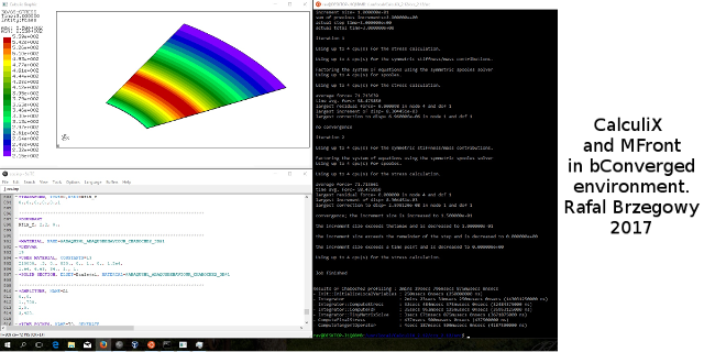
After Visual Studio, Mingw and Cygwin, there is a new
way to get MFront working on Windows !
Rafal Brzegowy have successfully compiled and tested
MFront using the Windows
Subsystem for LinuX (WSL). He was able to
use MFront generated behaviours with CalculiX delivered by the
bConverged
suite.
All tests worked, except some tests related to the
long double support in WSL.
TFEL and MFront now have their official
twitter account !
We will use it to spread various events and developments make in
TFEL and MFront.
MFront and Salome-Meca
(1/08/2017)Thanks to Jordi Alberich, a spanish introduction to
MFront and Salome-Meca is available here:
http://tfel.sourceforge.net/tutorial-spanish.html
The talks of the third MFront Users Day are available here:
https://github.com/thelfer/tfel-doc
Cast3M 2017 has
been released.
A binary version of TFEL compiled for Cast3M 2017 is now available for download on sourceforge:
https://sourceforge.net/projects/tfel/files/
MTestArbitrary non linear constraints can be now imposed in
MTest using @NonLinearConstraint keyword.
Abritray non linear constraints can be used to:
A constraint \(c\) is imposed by introducing a Lagrange multiplier \(\lambda\).
Consider a small strain elastic behaviour characterised by its free energy \(\Psi\). In the only loading is the constraint \(c\), the solution satisfies: \[ \underset{\underline{\varepsilon},\lambda}{\min}\Psi-\lambda\,c \]
In this case, the constraint \(c\) is equivalent to the following imposed stress:
\[ -\lambda\,{\displaystyle \frac{\displaystyle \partial c}{\displaystyle \partial \underline{\varepsilon}}} \]
If the constraint is \(\sigma_{xx}-\sigma_{0}\), where \(\sigma_{0}\) is a constant value, the previous equation shows that imposing this constraint is not equivalent to imposing an uniaxial stress state \(\left(\sigma_{xx}\,0\,0\,0\,0\,0\right)\).

The implementation of an an isotropic viscoplastic behaviour with several kinematic variables following the Amstrong-Frederic evolution law is described here
The behaviour is described by a standard split of the strain \(\underline{\varepsilon}^{\mathrm{to}}\) in an elastic and a plastic parts, respectively denoted \(\underline{\varepsilon}^{\mathrm{el}}\) and \(\underline{\varepsilon}^{\mathrm{vis}}\):
\[ \underline{\varepsilon}^{\mathrm{to}}=\underline{\varepsilon}^{\mathrm{el}}+\underline{\varepsilon}^{\mathrm{vis}} \]
The stress \(\underline{\sigma}\) is related to the the elastic strain \(\underline{\varepsilon}^{\mathrm{el}}\) by a the standard Hooke behaviour:
\[ \underline{\sigma}= \lambda\,{\mathrm{tr}{\left(\underline{\varepsilon}^{\mathrm{el}}\right)}}\,\underline{I}+2\,\mu\,\underline{\varepsilon}^{\mathrm{el}} \]
The viscoplastic behaviour follows a standard viscoplastic behaviour: \[ \underline{\dot{\varepsilon}}^{\mathrm{vis}}=\left\langle{{\displaystyle \frac{\displaystyle F}{\displaystyle K}}}\right\rangle^{m}\,\underline{n}=\dot{p}\,\underline{n} \]
where \(F\) is the yield surface defined below, \(<.>\) is Macaulay brackets, \(\underline{n}\) is the normal to \(F\) with respect to the stress and \(p\) is the equivalent plastic strain.
The yield surface is defined by: \[ F{\left(\underline{\sigma},\underline{X}_{i},p\right)}={\left(\underline{\sigma}-\sum_{i=1}^{N}\underline{X}_{i}\right)}_{\mathrm{eq}}-R{\left(p\right)}=s^{e}_{\mathrm{eq}}-R{\left(p\right)} \]
where:
We have introduced an effective deviatoric stress \(\underline{s}^{e}\) defined by: \[ \underline{s}^{e}=\underline{s}-\sum_{i=1}^{N}\underline{X}_{i} \] where \(\underline{s}\) is the deviatoric part of the stress.
The normal is then given by: \[ \underline{n}={\displaystyle \frac{\displaystyle \partial F}{\displaystyle \partial \underline{\sigma}}}={{\displaystyle \frac{\displaystyle 3}{\displaystyle 2}}}\,{{\displaystyle \frac{\displaystyle \underline{s}^{e}}{\displaystyle s^{e}_{\mathrm{eq}}}}} \]
The isotropic hardening is defined by: \[ R{\left(p\right)}=R_{\infty} + {\left(R_{0}-R_{\infty}\right)}\,\exp{\left(-b\,p\right)} \]
\[ \underline{X}_{i}={{\displaystyle \frac{\displaystyle 2}{\displaystyle 3}}}\,C_{i}\,\underline{a}_{i} \]
The evolution of the kinematic variables \(\underline{a}_{i}\) follows the Armstrong-Frederic rule:
\[ \underline{\dot{a}}_{i}=\underline{\dot{\varepsilon}}^{\mathrm{vis}}-g[i]\,\underline{a}_{i}\,\dot{p}=\dot{p}\,{\left(\underline{n}-g[i]\,\underline{a}_{i}\right)} \]

CEA and EDF are pleased to announce that the third MFront users meeting will take place on May 30th 2017 and will be organized by CEA DEC/SESC at CEA Saclay in the DIGITEO building (building 565, room 34).
Researchers and engineers willing to present their works are welcome.
They may contact the organizers for information at: .
Registration by sending an email at the previous address before May 12th is required to ensure proper organization.
tfel-plot project
The tfel-plot project is meant to create:
C++11 library for generating 2D plots
based on the Qt library (version 4 or version 5).gnuplot called
tplot.This project is based on:
TFEL
libraries.Qt framework
.Compared to gnuplot, we wanted to introduced the
following new features:
tplot from the command line.Qt code.C functions in shared libraries,
such a the ones generated by the MFront code
generator.TFEL project
such as:
diff
operator.More details can be found on the dedicated github
page:
https://github.com/thelfer/tfel-plot
A new example has been added in the gallery here.
This example describes a simple orthotropic behaviour.
The behaviour is described by a standard split of the strain \(\underline{\varepsilon}^{\mathrm{to}}\) in an elastic and a plastic parts, respectively denoted \(\underline{\varepsilon}^{\mathrm{el}}\) and \(\underline{\varepsilon}^{\mathrm{p}}\):
\[ \underline{\varepsilon}^{\mathrm{to}}=\underline{\varepsilon}^{\mathrm{el}}+\underline{\varepsilon}^{\mathrm{p}} \]
The stress \(\underline{\sigma}\) is related to the the elastic strain \(\underline{\varepsilon}^{\mathrm{el}}\) by a the orthotropic elastic stiffness \(\underline{\underline{\mathbf{D}}}\):
\[ \underline{\sigma}= \underline{\underline{\mathbf{D}}}\,\colon\,\underline{\varepsilon}^{\mathrm{el}} \]
The plastic part of the behaviour is described by the following yield surface: \[ f{\left(\sigma_{H},p\right)} = \sigma_{H}-\sigma_{0}-R\,p \]
where \(\sigma_{H}\) is the Hill stress defined below, \(p\) is the equivalent plastic strain. \(\sigma_{0}\) is the yield stress and \(R\) is the hardening slope.
The Hill stress \(\sigma_{H}\) is defined using the fourth order Hill tensor \(H\): \[ \sigma_{H}=\sqrt{\underline{\sigma}\,\colon\,\underline{\underline{\mathbf{H}}}\colon\,\underline{\sigma}} \]
The plastic flow is assumed to be associated, so the flow direction \(\underline{n}\) is given by \({\displaystyle \frac{\displaystyle \partial f}{\displaystyle \partial \underline{\sigma}}}\):
\[ \underline{n} = {\displaystyle \frac{\displaystyle \partial f}{\displaystyle \partial \underline{\sigma}}} = {{\displaystyle \frac{\displaystyle 1}{\displaystyle \sigma_{H}}}}\,\underline{\underline{\mathbf{H}}}\,\colon\,\underline{\sigma} \]
The default eigen solver for symmetric tensors used in
TFEL is based on analitical computations of the eigen
values and eigen vectors. Such computations are more efficient but less
accurate than the iterative Jacobi algorithm (see [8, 9]).
With the courtesy of Joachim Kopp, we have introduced the following algorithms:
The implementation of Joachim Kopp have been updated for
C++-11 and make more generic (support of all the floatting
point numbers, different types of matrix/vector objects). The algorithms
have been put in a separate namespace called fses (Fast
Symmetric Eigen Solver) and is independant of the rest of
TFEL.
We have also introduced the Jacobi implementation of the
Geometric Tools library (see [10,
11]).
Those algorithms are available in 3D. For 2D symmetric tensors, we fall back to some default algorithm as described below.
| Name | Algorithm in 3D | Algorithm in 2D |
|---|---|---|
TFELEIGENSOLVER |
Analytical (TFEL) | Analytical (TFEL) |
FSESJACOBIEIGENSOLVER |
Jacobi | Analytical (FSES) |
FSESQLEIGENSOLVER |
QL with implicit shifts | Analytical (FSES) |
FSESCUPPENEIGENSOLVER |
Cuppen’s Divide & Conquer | Analytical (FSES) |
FSESANALYTICALEIGENSOLVER |
Analytical | Analytical (FSES) |
FSESHYBRIDEIGENSOLVER |
Hybrid | Analytical (FSES) |
GTESYMMETRICQREIGENSOLVER |
Symmetric QR | Analytical (TFEL) |
The various eigen solvers available are enumerated in Table 1.
The eigen solver is passed as a template argument of the
computeEigenValues or the computeEigenVectors
methods as illustrated in the code below:
tmatrix<3u,3u,real> m2;
tvector<3u,real>    vp2;
std::tie(vp,m)=s.computeEigenVectors<Stensor::GTESYMMETRICQREIGENSOLVER>();| Algorithm | Failure ratio | \(\Delta_{\infty}\) | Times (ns) | Time ratio |
|---|---|---|---|---|
TFELEIGENSOLVER |
0.000632 | 7.75e-14 | 252663338 | 1 |
GTESYMMETRICQREIGENSOLVER |
0 | 2.06e-15 | 525845499 | 2.08 |
FSESJACOBIEIGENSOLVER |
0 | 1.05e-15 | 489507133 | 1.94 |
FSESQLEIGENSOLVER |
0.000422 | 3.30e-15 | 367599140 | 1.45 |
FSESCUPPENEIGENSOLVER |
0.020174 | 5.79e-15 | 374190684 | 1.48 |
FSESHYBRIDEIGENSOLVER |
0.090065 | 3.53e-10 | 154911762 | 0.61 |
FSESANALYTICALEIGENSOLVER |
0.110399 | 1.09e-09 | 157613994 | 0.62 |
We have compared the available algorithm on \(10^{6}\) random symmetric tensors whose components are in \([-1:1]\).
For a given symmetric tensor, we consider that the computation of the eigenvalues and eigenvectors failed if: \[ \Delta_{\infty}=\max_{i\in[1,2,3]}\left\|\underline{s}\,\cdot\,\vec{v}_{i}-\lambda_{i}\,\vec{v}_{i}\right\|>10\,\varepsilon \] where \(\varepsilon\) is the accuracy of the floatting point considered.
The results of those tests are reported on Table 2:
TFEL offers a very interesting compromise between accuracy
and numerical efficiency.FSESJACOBIEIGENSOLVER eigen solver is a good choice.TFEL for FreeBSD (20/01/2017)
Thanks to the work of Pedro F. Giffuni , an official port of
TFEL/MFront is available for FreeBSD:
http://www.freshports.org/science/tfel/
To install an executable package, you can now simply do:
pkg install tfel-mfrontAlternativel, to build and install TFEL from the ports
tree, one can do:
cd /usr/ports/science/tfel/
make
make installThe implementation of the Ogden behaviour is now described in depth in the following page:
http://tfel.sourceforge.net/ogden.html
This behaviour is interesting as it highlights the features
introduced in TFEL-3.0 for computing isotropic functions of
symmetric tensors.
This page uses the formal developments detailled in:
http://tfel.sourceforge.net/hyperelasticity.html
Concerning hyperviscoelasticity, a page describing a generic implementation is available here:
http://tfel.sourceforge.net/hyperviscoelasticity.html
If you have particular wishes on behaviours implementation that you would like to see treated, do not hesitate to send a message at .
A page referencing examples of well written mechanical behaviours has been created here:
http://tfel.sourceforge.net/gallery.html
For each behaviours, we will try to provide tutorial-like pages
explaining the implementations details (usage of tensorial objects,
special functions of the TFEL library, choice of the
algorithms, and so on…)
The first attempt is an hyperelastic behaviour already available in
Code_Aster: the Signorini behaviour. You can find the page
here:
http://tfel.sourceforge.net/signorini.html
This is still under review, so corrections and feed-backs would be greatly appreciated. The following behaviours are planned to be addressed:
If you have particular wishes on behaviours implementation that you would like to see treated, do not hesitate to send a message at .
From a user point of view, TFEL 3.0 brings many game-changing features:
Europlexus, Abaqus/Standard,
Abaqus/Explicit, CalculiX)MTest.C++ and python which allow building
external tools upon MFront and MTest. This
point is illustrated by the development by EDF MMC in the Material
Ageing Plateform of a new identification tool which is particularly
interesting.Many improvements for mechanical behaviours have also been made:
@ComputeStiffnessTensor,
@ComputeThermalExpansion, @Swelling,
@AxialGrowth, @HillTensor etc..).fortran03, java,
GNU/Octave).A detailed version of the release notes is available here.
UnilateralMazars (1
June 2016)
A new behaviour implementation has been submitted by F. Hamon (EDF R&D AMA). This behaviour describes the damaging behaviour of concrete with unilateral effects as described in a dedicated paper:
A new 3D damage model for concrete under monotonic, cyclic and dynamic loadings. Jacky Mazars, François Hamon and Stéphane Grange. Materials and Structures ISSN 1359-5997 DOI 10.1617/s11527-014-0439-8
This implementation can be found in the current development sources of MFront.
The Abaqus Explicit interface is becoming quite usable du to the extensive testing efforts of D. Deloison (Airbus). Here is an example a punching test (This test was also modelled using Abaqus Standard).
@Brick "StandardElasticity";Behaviour bricks will be one of the most important new feature of
TFEL 3.0.
A dedicated page has been created here
EUROPLEXUS interface (27 May 2016)
An interface for the EUROPLEXUS explicit finite element solver has been developed.
EUROPLEXUS (EPX) is a simulation software dedicated to the analysis of fast transient phenomena involving structures and fluids in interaction.
See the dedicated page for more information.
tfel-doc
github repository. Talks of the Second MFront Users Day (27
May 2016)A github repository has been set up to store various
documents describing TFEL and MFront usage. The talks of the first and
second MFront Users Days are available there:
https://github.com/thelfer/tfel-doc
github
repository (27 May 2016)The subversion repository used by CEA and EDF are now
synchronized with a public githbub repository:
https://github.com/thelfer/tfel
All the branches, commit description and history of TFEL are available. This repository is read-only. Its purpose is to integrate TFEL in continous-integration projects which depends on TFEL.
mfront module (May 2016)A new python module has been introduced to analyse
MFront files.
An overview of the module is available here.
Here is a typical usage example:
import mfront

dsl = mfront.getDSL("Chaboche.mfront")
dsl.setInterfaces(["aster"])
dsl.analyseFile("Chaboche.mfront",[])

# file description
fd = dsl.getFileDescription()
print("file author:      ", fd.authorName)
print("file date:        ", fd.date)
print("file descrption:\n", fd.description)

# targets information
tgt = dsl.getTargetsDescription()

# loop over (to be) generated libraries
for l in tgt:
    print(l)
Cast3M 2016 has
been released.
This version allow even better integration with MFront
and can now directly be used to make direct calls to MFront
libraries for material properties (mechanical behaviours can be used
since Cast3M 2015).
This syntax is now officially supported:
Ty = 'TABLE' ;
Ty.'LIB_LOI'   = 'libCastemM5.so' ;
Ty.'FCT_LOI'   = 'M5_YoungModulus' ;
Ty.'VARIABLES' = 'MOTS' 'T';

mo = 'MODELISER' m 'MECANIQUE' 'ELASTIQUE';
ma = 'MATERIAU' mo 'YOUN' Ty 'NU' 0.3;
A binary version of TFEL compiled for Cast3M 2016 is now available for download on sourceforge:
https://sourceforge.net/projects/tfel/files/

CEA and EDF are pleased to announce that the second MFront users meeting will take place on May 20th 2016 and will be organized by EDF R&D at the EDF Lab Paris Saclay location.
Researchers and engineers willing to present their works are welcome. They may contact the organizers for information at: .
This users day will take place on Friday, May 20th, 2016 at EDF Lab Paris-Saclay (access map).
Registration is required to ensure proper organization. See the dedicated form on the Code_Aster website: http://www.code-aster.org/spip.php?article906
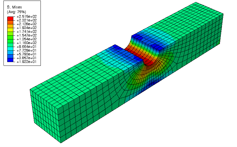
The current development version now includes an experimental
interface to the Abaqus
solver through the umat subroutine.
The following results shows the results obtained on notched beam
under a cyclic loading with an isotropic hardening plastic beahviour
implemented with mfront:
The mfront results can be compared to the results
obtained using Abaqus in-built model on the following
figure:
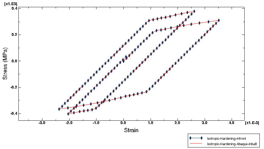
The Abaqus interface is still in its early stage of
developments. A full description of its usage and current abilities can
be found in the associated documentation.
Feed-back from users would be greatly welcomed.
An IMSIA seminar about MFront will be held on Januar, 27 2016. Here is the official announcement (in french):
Séminaire IMSIA : Implémentation de lois de comportement mécanique à l’aide du générateur de code MFront
Créé dans le cadre de la simulation des éléments combustibles nucléaire au sein d’une plate-forme logicielle nommée PLEIADES, MFront est un générateur de code, distribué en open-source [1], qui vise à permettre aux ingénieurs/chercheurs d’implémenter de manière simple et rapide des lois de comportements mécaniques de manière indépendante du code cible (EF ou FTT) [2,3].
Ce dernier point permet d’échanger les lois MFront entre différents partenaires, universitaires ou industriels. Le lien vers les codes cible se fait via la notion d’interface. A l’heure actuelle, des interfaces existent pour les codes Cast3M, Code-Aster, Abaqus, ZeBuLoN, AMITEX_FFT et d’autres codes métiers, et sont en cours de développement pour d’autres codes tels Europlexus, …
Ce séminaire proposera une description des fonctionnalités de MFront (lois en transformations infinitésimales et en grandes transformations, modèles de zones cohésives) et commentera plusieurs exemples d’applications, discutera des performances numériques obtenues et soulèvera la question de la portabilité des connaissances matériau. Nous montrerons qu’une démarche cohérente allant des expérimentations aux codes de calcul est nécessaire.
[1] http://tfel.sourceforge.net
[2] Introducing the open-source mfront code generator: Application to mechanical behaviours and material knowledge management within the PLEIADES fuel element modelling platform. Thomas Helfer, Bruno Michel, Jean-Michel Proix, Maxime Salvo, Jérôme Sercombe, Michel Casella, Computers & Mathematics with Applications, Volume 70, Issue 5, September 2015, Pages 994-1023, ISSN 0898-1221, http://dx.doi.org/10.1016/j.camwa.2015.06.027.
[3] Implantation de lois de comportement mécanique à l’aide de MFront : simplicité, efficacité, robustesse et portabilité. T. Helfer, J.M. Proix, O. Fandeur. 12ème Colloque National en Calcul des Structures 18-22 Mai 2015, Giens (Var)
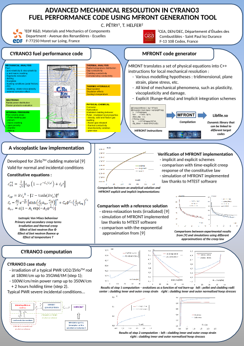
A poster describing the use of MFront in EDF
Cyrano3 fuel performance code has been presented at the LWR
Fuel Performance Meeting 2015 (13 - 17 September 2015, Zurich,
Switzerland):
Version 2.0.3 is mostly a bug-fix release:
CxxTokenizer class which was
appears when using the clang
libc++ standard library. This prevented many
MTest tests to work on Mac OS X.ExternalBehaviourDescription was
introducedAxialGrowth entry was added to the glossaryA full description of the 2.0.3 release can be found here (in french).
mfront-doc (19 August 2015)mfront-doc allows the user to extract the documentation
out of MFront file. mfront-doc generates files
in pandoc markdown
format. Those files can be processed using pandoc and be converted to
one of the many file format supported by pandoc, including LaTeX, html
or various Word processor formats: Microsoft Word docx,
OpenOffice/LibreOffice ODT.
mfront-doc is developped in the 3.0.x branche of
TFEL. A overview of the mfront-doc
functionalities can be found here.
New documentation pages were added to describe the MTest
and MFront keywords:
MFront keywords, sorted by domain specific languages:
MTest keywordsThe current development version of MFront includes two
new interfaces for material properties:
java designed for the java
language.octave designed for GNU Octave
which is a high-level interpreted language, primarily intended for
numerical computations.Here is an example of a GNU Octave
session used to compute the Young Modulus of uranium-plutonium carbide
\(UPuC\) for various porosities over a
range of temperatures:
octave:1> T=[300:100:1500]
T =
    300    400    500    600    700    800    900   1000   1100   1200   1300   1400   1500
octave:2> y01=UPuC_YoungModulus(T,0.1)
y01 =
   1.7025e+11   1.6888e+11   1.6752e+11   1.6616e+11   1.6480e+11   1.6344e+11   1.6207e+11   1.6071e+11   1.5935e+11   1.5799e+11   1.5662e+11   1.5526e+11   1.5390e+11
octave:3> y02=UPuC_YoungModulus(T,0.2)
y02 =
1.1853e+11 1.1758e+11 1.1663e+11 1.1568e+11 1.1474e+11 1.1379e+11 1.1284e+11 1.1189e+11 1.1094e+11 1.0999e+11 1.0905e+11 1.0810e+11 1.0715e+11The number of papers in which MFront is used is
increasing. A dedicated page has been added here.
If you publish papers which refers to MFront, please
consider contributing to this page.
The first paper dedicated to MFront, written by Thomas
Helfer, Bruno Michel, Jean-Michel Proix, Maxime Salvo, Jérôme Sercombe,
and Michel Casella, has been accepted Computers and Mathematics with
Applications. The paper is available online on the sciencedirect
website:
http://www.sciencedirect.com/science/article/pii/S0898122115003132
The PLEIADES software environment is devoted to the thermomechanical simulation of nuclear fuel elements behaviour under irradiation. This platform is co-developed in the framework of a research cooperative program between Électricité de France (EDF), AREVA and the French Atomic Energy Commission (CEA). As many thermomechanical solvers are used within the platform, one of the PLEAIADES’s main challenge is to propose a unified software environment for capitalisation of material knowledge coming from research and development programs on various nuclear systems.
This paper introduces a tool called mfront which is basically a code generator based on C++ (Stroustrup and Eberhardt, 2004). Domain specific languages are provided which were designed to simplify the implementations of new material properties, mechanical behaviours and simple material models. mfront was recently released under the GPL open-source licence and is available on its web site: http://tfel.sourceforge.net/.
The authors hope that it will prove useful for researchers and engineers, in particular in the field of solid mechanics. mfront interfaces generate code specific to each solver and language considered.
In this paper, after a general overview of mfront functionalities, a particular focus is made on mechanical behaviours which are by essence more complex and may have significant impact on the numerical performances of mechanical simulations. mfront users can describe all kinds of mechanical phenomena, such as viscoplasticity, plasticity and damage, for various types of mechanical behaviour (small strain or finite strain behaviour, cohesive zone models). Performance benchmarks, performed using the Code-Aster finite element solver, show that the code generated using mfront is in most cases on par or better than the behaviour implementations written in fortran natively available in this solver. The material knowledge management strategy that was set up within the PLEIADES platform is briefly discussed. A material database named sirius proposes a rigorous material verification workflow.
We illustrate the use of mfront through two case of studies: a simple FFC single crystal viscoplastic behaviour and the implementation of a recent behaviour for the fuel material which describes various phenomena: fuel cracking, plasticity and viscoplasticity.

Cast3M 2015 has
been released.
This release allow direct call to MFront libraries for
mechanical behaviours. The following syntax of the
MODELISER operator is now officially supported:
mod1 = 'MODELISER' s1 'MECANIQUE' 'ELASTIQUE' 'ISOTROPE'
   'NON_LINEAIRE' 'UTILISATEUR'
   'LIB_LOI' 'src/libUmatBehaviour.so'
   'FCT_LOI' 'umatnorton'
   'C_MATERIAU' coel2D
   'C_VARINTER' stav2D
   'PARA_LOI'   para2D
   'CONS' M;
See the dedicated page for more information.
Salome-Meca
2015.1 is out (1O April 2015)
Salome-Meca 2015.1, which combines the Salome platform
and Code-Aster,
has been released on 1O April 2015. This version is the first to include
a pre-packaged version of TFEL (version 2.0.1).
Salome-Meca
and Code_Aster Users Day (26 March 2015)
A presentation of MFront was done during the
Salome-Meca and Code_Aster Users Day 2015 user
meeting at EDF Lab Clamart.
Slides can be found here.
MFront user
meeting (6 Februar 2015)The first MFront user meeting was held in Cadarache on
Februar,6 2015. 27 participants from CEA, EDF, Areva and CNRS could
discuss and comment about their use of MFront.
Various subjects were discussed:
TFEL/MFront 2.0Code-Aster development teamCyrano3 development teamMFrontTFEL 3.xThose talks are available here
MFront user meeting (12 December 2014)We are glad to announce that the first MFront user
meeting will be held in Cadarache on Februar,6 2015. Everyone is invited
but a registration must be performed before Januar, 16 2015 ().
Various subjects are already planned:
TFEL/MFront 2.0Code-Aster development teamCyrano3 development teamMFront usage for concrete modellingMFront usage in finite strain analysesMFront to nuclear fuel modellingOther talks are welcomed.
MFront at the Cast3M user meeting (4
December 2014)
The Cast3M user
meeting was held in Paris on November 28, 2014. Jérémy Hure had a talk
about the application of MFront in finite strain
elasto-plasticity. This talk is available here.
AMITEX_FFTP
has its own website (4 December 2014)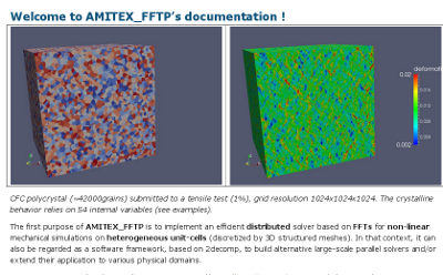
AMITEX_FFTP
has now its own dedicated
webiste.
The main purpose of AMITEX_FFTP
is to implement an efficient distributed mechanical solver based on Fast
Fourier Transform. AMITEX_FFTP
is developped by CEA in the Departement of Nuclear Material.
AMITEX_FFTP
is distributed under a free license for research and education
purpose.
TFEL version 2.0.1 is now available. This is mainly a
bug-fix release after version 2.0.0.
This version is meant to be used in Code-Aster version 12.3 that will be released in January 2015.
A new contact address has been created: .
This address can be used to contact directly the developers of
TFEL and MFront for specific issues. However,
if your issue may interest a broader audience, you may want to send a
post to the TFEL users mailing lists: .
MFront
talk at Materiaux 2014 Montpellier (24 November 2014)
An MFront talk was given at Materiaux 2014. Slides (in
french) are available here.
Windows 64bits and
Cast3M 2014 (18 November 2014)
A beta version of tfel-2.0.1 for Windows 64bits and Cast3M
2014 has been released. A binary installer is provided here.
Installing this version requires a functional installation of Cast3M \(2014\) (which shall be patched to call external
libraries) and the MSYS shell (It is recommended not to
install mingw compilers along with the MSYS
shell as Cast3M
provides its own version of those compilers).
Installation instructions of those requirements are available here.
Any feedback would be gratefully acknowledge.
Note: The binary provided requires the
mingw libraries delivered with Cast3M
2014.
Note: A standalone version of tfel-2.0.1 will be provided shortly.
MFront
behaviours can now be used in AMITEX_FFTP (24 October
2014)AMITEX_FFTP is a massively parallel mechanical solver
based on FFT developed at CEA. MFront behaviours can be
used in AMITEX_FFTP through the UMAT interface
introduced by the Cast3M finite element
solver.
 voxels)")
TFEL/MFront
on Cast3M web site
(15 October 2014)A page
dedicated to MFront is now available on the Cast3M web site.

Here is the official announcement by Jean-Paul DEFFAIN (in French):
Bonjour,
Une version libre de MFront est désormais officiellement disponible sous licence GPL et CECILL-A.
Cette version 2.0 permet entre autres de générer des lois de comportements en transformations infinitésimales et en grandes transformations ainsi que des modèles de zones cohésives. Les lois générées sont utilisables dans les codes aux éléments finis Cast3M, Code-Aster, ZeBuLoN, l’ensemble des applications développées dans la plateforme PLEIADES, notamment Cyrano3, et le solveur FFT de la plate-forme. Des interfaces vers d’autres codes peuvent être rajoutées.
Un projet dédié a été crée sur sourceforge (http://sourceforge.net/projects/tfel) et fournit :
- un site dédié (http://tfel.sourceforge.net)
- un espace de téléchargement (http://sourceforge.net/projects/tfel/files) qui permet d’accéder à la version 2.0
- les listes de diffusion tfel-announce et tfel-discuss (http://sourceforge.net/p/tfel/tfel)
- un forum (http://sourceforge.net/p/tfel/discussion)
- un outil de demande d’évolution et de déclaration de bugs par tickets (http://sourceforge.net/p/tfel/tickets)
Pour les personnes souhaitant contribuer au développement, le dépôt subversion est accessible sur le serveur:
https://svn-pleiades.cea.fr/SVN/TFEL
L’accès à ce dépôt est restreint mais nécessite l’ouverture d’un compte spécifique sur demande au .
Nous remercions chaleureusement tous ceux qui ont contribué à cette version et invitons toutes les personnes intéressées à se joindre au développement de MFront.
Jean-Paul DEFFAIN
Chef du programme SIMU
Commissariat à l’Énergie Atomique