 and the von Mises stress in plane stress")
TFEL, MFront and MTestMFrontGallery projectMFrontDDIF2
brick@StrainMeasure
keywordWindows operating systemTravis CI and
Appveyor continous integration servicesTFEL
libraries
MFront code generator
MTest solver
mfront-query tool
tfel-config toolmfm
toolImplicitDSL: Detect non finite values during
resolutionMTest:
check if the residual is finite and not NaNNaN values in material propertiesUMAT++ interfacemfront python modulepython bindings for the mtest::Behaviour
classpython bindings for the
mfront::BehaviourDescription classmtest::Behaviour classmfront-querymfront-queryMieheApelLambrechtLogarithmicStrain finite strain
strategy@FiniteStrainStrategy keyword. Deprecate definition of the
finite strain strategies in the interfaces.@ElasticMaterialProperties does not work for DSL describing
isotropics behavioursmfront-query: handle static variablespython bindings for the SearchPathsHandler
class in the mfront moduleThe page declares the new functionalities of the 3.1 version of the
TFEL project.
The TFEL project is a collaborative development of CEA and EDF
dedicated to material knowledge manangement with special focus on
mechanical behaviours. It provides a set of libraries (including
TFEL/Math and TFEL/Material) and several
executables, in particular MFront and
MTest.
TFEL is available on a wide variety of operating systems
and compilers.
MFrontGallery projectThe MFront gallery is meant to present well-written
implementation of behaviours that will be updated to follow
MFront latest evolutions. In each case, the integration
algorithm is fully described.
The MFrontGallery project is a cmake
project which builds material libraries for all the codes and/or
languages supported by MFront based on the implementation
described in the gallery. The purpose of this project is twofold:
MFront files, including lots of useful cmake
macros, recipes to build shared libraries and add tests.The MFrontGallery project is available as a
github repository: https://github.com/thelfer/MFrontGallery
The implementation of various hyperelastic behaviours can be found here:
The following page describes how to implement standard hyperviscoelastic behaviours based on the development in Prony series:
http://tfel.sourceforge.net/hyperviscoelasticity.html
This following article shows how to implement an isotropic viscoplastic behaviour combining isotropic hardening and multiple kinematic hardenings following an Armstrong-Frederic evolution of the back stress:
http://tfel.sourceforge.net/isotropicplasticityamstrongfrederickinematichardening.html
The TFEL/Material provides functions to handle advanced
yield criteria, such as:
Following Scherzinger (see [3] for details), special care has been taken to avoid overflow in the evaluation of the yield stress.
Those two yield criteria are based on the eigenvalues and of the stress. The computation of the second derivative, required to build the jacobian of the implicit system, is thus quite involved.
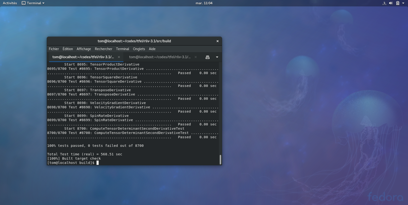
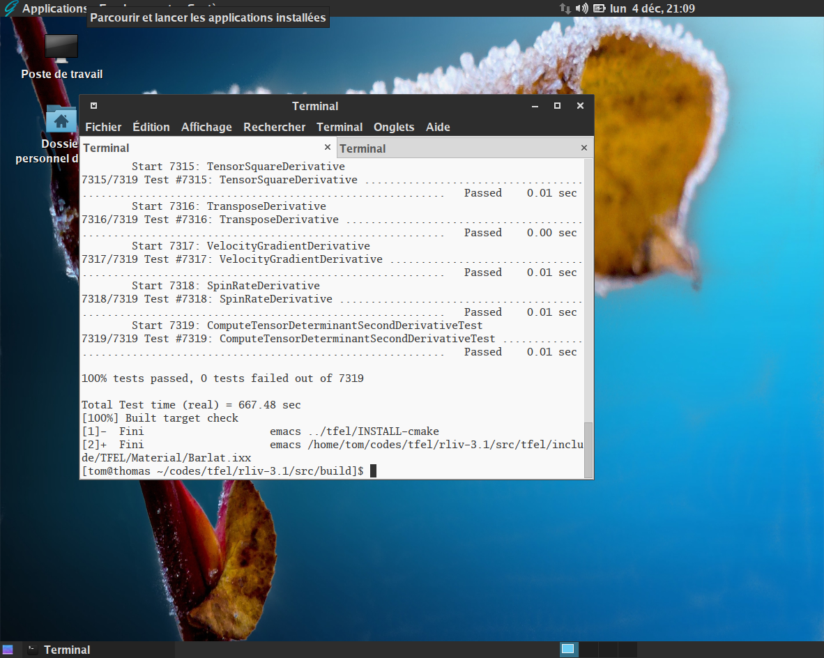
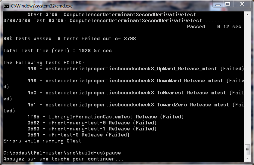
This release has seen lot of work in the overall numerical
reproducibility and stability of TFEL algorithms and lead
to duplicate most of tests, who are now run using different rounding
modes.
Tests based on mtest are run \(5\) times, one for each of the four
rounding modes defined in the IEEE754 norm, plus one time
using a specific mode which randomly switches between those modes at
various stages of the computations.
Although very crude with respect to advanced approaches such as the
CADNA library (see [5]) or the
verrou software, developped by EDF on top of
valgrind (see [6]), those checks, combined
with demanding convergence criteria, have proven to be helpful and led
to several developments: see for example the section 2.3.1.2 which
compares various algorithms to find the eigen vectors of symmetric
tensors.
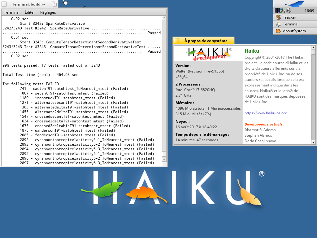
Note
Old versions of the
libmlibrary (such as the one package withDebianWheezyand those found on some exotic systems, such asHaiku), do not support working in other rounding mode than the default one (rounding to the nearest) and can crash (segfaults !).Disabling changing the rounding mode on those systems can be specified by passing
-DTFEL_BROKEN_LIB_MATH=ONtocmake.
-ffast-math with GCC an
clangOne side effect of the work on the enhanced numerical stability is
that the -ffast-math flag of GCC and
clang can now be enabled more safely. This significantly
improve the performances of the generated code by allowing optimizations
that do not preserve strict IEEE compliance. For instance, the overall
tests delivered with TFEL runs almost \(10\,\%\) faster with this option
enabled.
Most of those optimizations are used by default by the
Intel compiler.
There are two potential issues with this flags:
TFEL/MFront, it has been seen that the
algorithm used to compute the eigenvalues and the eigenvectors of
symmetric tensors can be affected. New algorithms, more stable but less
efficient, have been introduce, as discussed below.GCC, various mathematical functions of the
standard library behaves in an unexpected manner and can not be trusted.
For example, the isnan function returns true,
even if its argument is NaN. This issue has been overcome
by implementing proper versions of the fpclassify,
isnan, isfinite functions, as described below
in paragraph 2.3.3.To build TFEL with the -ffast-math, just
pass the -Denable-fast-math=ON option to
cmake.
Note
Even if
TFELis not built with the-ffast-math, this option can be used to compileMFrontfiles, by specifying the--obuild=level2option toMFront, as follows:$ mfront --obuild=level2 --interface=....
MFrontSupport for writting single crystal behaviours have been greatly
improved thanks to the TFELNUMODIS library, which borrows
code for the NUMODIS project.
The following new keywords are now available in
MFront:
@CrystalStructure. The following crystal structures are
supported:
Cubic: cubic structure.BCC: body centered cubic structure.FCC: face centered cubic structure.HCP: hexagonal closed-packed structures.@SlidingSystem,
@GlidingSystem or @SlipSystem. Several slip
systems families ca be defined by @SlidingSystems,
@GlidingSystems or @SlipSystems.@InteractionMatrix keyword and is meant to describe the
effect of dislocations on hardening.@DislocationsMeanFreePathInteractionMatrix keyword and is
meant to evaluate the effect of all the dislocations on the mean free
path of dislocations of a specific system.Those keywords are fully documented on this page. As most of the information
relative to the slip system and the interaction matrix are automatically
generated, the use of the mfront-query tool is strongly
advised.
DDIF2
brickDDIF2 is the name of a description of damage which
formulation is inspired by softening plasticity. This description is the
basis of most mechanical behaviour used in CEA’ fuel performance.
The DDIF2 brick can be used in place of the
StandardElasticity brick. Internally, the
DDIF2 brick is derived from the
StandardElasticity brick, so the definition of the elastic
properties follows the same rules.
This description is currently limited to initially isotropic
behaviours, but the damage is described in three orthogonal directions.
Those directions are currently fixed with respect to the global system.
For \(2D\) and \(3D\) modelling hypotheses, those directions
are determined by a material property, which external name is
AngularCoordinate, giving the angular coordinate in a
cylindrical system.
The description of damage is based on the following material properties:
fracture_stress option is used, the fracture
stresses are equal in each directions.fracture_stresses keyword can be used to
describe the fracture stresses in each of the three directions.softening_slope option is used, the softening
slopes are equal in each directions.softening_slopes keyword can be used to
describe the softening slopes in each of the three directions.In each case, a material property must be given as a value or as an
external MFront file.
Following Hillerborg approach (see [7]), softening slopes can
be related to fracture energies by the mesh size. Thus, rather than the
softening slopes, the user can provide the fracture energies through one
the fracture_energy or fracture_energies
options. In this case, an array of three material properties, which
external name is ElementSize, is automatically
declared.
The effect of external pressure on the crack surface can be taken
into account using the option
handle_pressure_on_crack_surface. If this option is true,
an external state variable called pr, which external name
is PressureOnCrackSurface, is automatically declared.
Here is an example of a behaviour based on the DDIF2
brick:
@DSL Implicit;
@Author Thomas Helfer;
@Date 25/10/2017;
@Behaviour DDIF2_4;

@Brick DDIF2 {
 fracture_stresses : {150e6,150e6,1e11},
 softening_slope : -75e9,
 handle_pressure_on_crack_surface : true
};
Here, the fracture stresses are different in each direction. The softening slope is the same in each direction. When a crack is open, the external pressure is applied on the crack surface.
@StrainMeasure
keywordIn previous versions of TFEL, the user would write
strain based behaviour. The definition of the strain, and by energetic
duality the definition of the stress, were not part of the
behaviour.
This is very important for a generic behaviour, which describe a physical phenomenon with no reference to a particular material, but it is not appropriate for a specific behaviour, identified for a specific material, because the definition of the strain is intrinsically part of the behaviour.
Three strain measure are currently supported:
The two first strain measures are suitable for use in finite strain analyses (including finite rotation), whereas the latter is limited to infinitesimal strain analyses (no rotation, small strain).
For the two first strain measures, the definition of the strain is done at a pre-processing stage, before calling the behaviour integration. The interpretation of the dual stress and its conversion to the stress measure expected by the solver is done after the behaviour integration, at a post-processing stage. During this post-processing stage, the consistent tangent operator is also converted to the one expected by the solver.
Those pre- and post-processing stages can be performed:
Code_Aster,
ZeBuLoN). In this case, the consistent use of the behaviour
was the responsability of the user.MFront interface (Cast3M,
Europlexus, CalculiX, etc.). In this case, one
has to use one following keywords:
@CastemFiniteStrainStrategy or
@CastemFiniteStrainStrategies for the Cast3M
interface. For backward compatibility, those keywords are synonymous of
@UmatFiniteStrainStrategy or
@UmatFiniteStrainStrategies.@EuroplexusFiniteStrainStrategy (or
@EPXFiniteStrainStrategy) for the Europlexus
interface.@AbaqusFiniteStrainStrategy for the
Abaqus/Standard and Abaqus/Explicit
interfaces.
Each case was quite error-prone and could lead to an improper usage of the behaviour.
To circumvent this issue, the @StrainMeasure keyword was
introduced. This keyword has two distinct effect, depending on the
interface:
Code_Aster), appropriate symbols are defined in the shared
library, so that the calling solver can deduce the appropriate strain
measure to be used.The TFEL_APPEND_VERSION option will append the version
number to the names of:
python
restriction on module’ names, the characters . and
- are replace by _ and that only the first
level modules are affected.share folder.This allows multiple executables to be installed in the same
directory. This option is available since TFEL version
\(3.0.2\)
The TFEL_VERSION_FLAVOUR let the user define a string
that will be used to modify the names of executables, libraries and so
on (see the previous paragraph for details).
For example, using -DTFEL_VERSION_FLAVOUR=dbg at the
cmake invocation, will generate an executable called
mfront-dbg.
This option can be combined with the TFEL_APPEND_VERSION
option.
Windows operating systemThere are various ways of getting TFEL and
MFront working on the the Windows operating
system:
Visual Studio
IDE and compilers suite. This is the de facto standard on the
Windows OS. This is also the compiler used by the Salome platform.
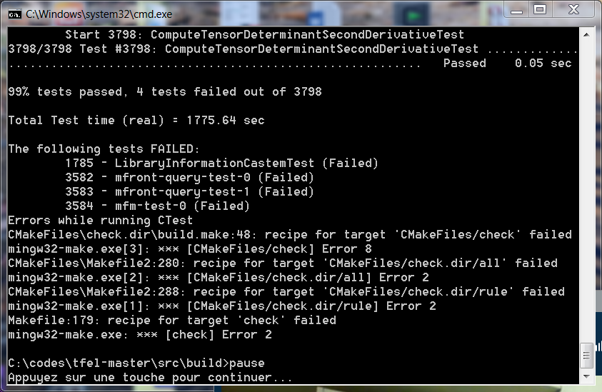
An installation guide for Visual Studio is available here.MINGW, which is a native
Windows port of the GNU Compiler Collection
(GCC). This port can be used in the MSYS)
environment. The Windows port of the Cast3M
finite element solver is built on the MINGW. An
installation guide for TFEL/MFront with
Cast3M 2017 is available
[here][http://tfel.sourceforge.net/install-windows-Cast3M2017.html). In
the MSYS environment, the compilation and installation
steps are similar to those in Linux. More details can be
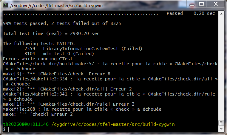
found here.TFEL/MFront under Cygwin, which provides a
large collection of GNU and Open Source tools which provide
functionality similar to a Linux distribution on
Windows and a substantial POSIX
API functionality. Various ports of the
CalculiX finite element solver is built upon
CygwinTFEL/MFront using one of the
Linux distribution available with the Windows Subsystem for LinuX.
This is not officially supported yet, but has been successfully tested
by various contributors.Visual Studio
supportSupport of the Visual Studio has been greatly improved.
TFEL versions 3.0.x could be compiled and
tested with Visual Studio 2015 and later, but
the resulting executables were not really usable by an end user. Indeed,
those versions of mfront could not generate a build system
compatible with Visual Studio.
For this reason, the cmake generator, described below in
section 3.1, has been introduced.
Two new interfaces were introduced in MFront:
CalculiX solver. Here native
is used to distinguish this interface from the
Abaqus/Standard interface which can also be used within
CalculiX. This interface can be used with
CalculiX 2.13.ANSYS APDL solver.
The latter is still experimental.Travis CI and
Appveyor continous integration servicesAs an open-source project available on
(github](https://github.com/thelfer/tfel), one have free
access to the Travis CI and Appveyor continous
integration services:
Travis CI allows us to build TFEL/MFront
on various combinations compilers (gcc and
clang) and operating systems (Ubuntu and
Mac Os).Appveyor allows us to build TFEL/MFront
with Visual Studio 2017.Since builds are limited a one hour, one can only test a subset of
the TFEL/MFront functionalities.
TFEL
librariesThe TFEL project provides several libraries. This
paragraph is about updates made in those libraries.
starts_with string algorithmThe starts_with string algorithm is an helper function
used to determine if a given string starts with another.
ends_with
string algorithmThe ends_with string algorithm is an helper function
used to determine if a given string ends with another.
LibraryInformation classThis release introduces the LibraryInformation class
that allow querying a library about exported symbols.
Note This class has been adapted from the
boost/dlllibrary version 1.63 and has been originally written by Antony Polukhin, Renato Tegon Forti and Antony Polukhin.
ExternalLibraryManager classIf a library is not found, the ExternalLibraryManager
class will try the following combinaisons:
lib in front of the library name (except for
Microsoft Windows platforms).lib in front of the library name and the
standard library suffix at the end (except for Microsoft
Windows platforms).The standard library suffix is:
.dll for Microsoft Windows
platforms..dylib for Apple MacOs
plateforms..so on all other supported systems.The getLibraryPath method returns the path to a shared
library:
GetModuleFileNameA function on
Windows which is reliable.Unix, no portable way exists, so the method simply
looks if the library can be loaded. If so, the method looks if the file
exists locally or in a directory listed in the
LD_LIBRARY_PATH variable.The ExternalLibraryManager class has several new methods
for better handling of behaviours’ parameters:
getUMATParametersNames returns the list of
parameters.getUMATParametersTypes returns a list of integers
which gives the type of the associated paramater: The integer values
returned have the following meaning:
getRealParameterDefaultValue,
getIntegerParameterDefaultValue, and
getUnsignedShortParameterDefaultValue methods allow
retrieving the default value of a parameter.The ExternalLibraryManager class has several new methods
for better handling of a behaviour’ variable bounds:
hasBounds,hasLowerBound and
hasUpperBound allow querying about the existence of bounds
for a given variable.getLowerBound method returns the lower bound a
variable, if defined.getUpperBound method returns the upper bound a
variable, if defined.The ExternalLibraryManager class has several new methods
for better handling of a behaviour’ variable bounds:
hasPhysicalBounds,hasLowerPhysicalBound and
hasUpperPhysicalBound allow querying about the existence of
bounds for a given variable.getLowerPhysicalBound method returns the physical
lower bound a variable, if defined.getUpperPhysicalBound method returns the physical
upper bound a variable, if defined.The getEntryPoints method returns a list containing all
mfront generated entry points. Those can be functions or classes
depending on the interface’s needs.
The getMaterialKnowledgeType allows retrieving the
material knowledge type associated with and entry point. The returned
value has the following meaning:
The getInterface method allows retrieving the interface
of used to generate an entry point. The value returned is defined by
MFront following Table 1.
| Finite element solver | MFront interface name |
|---|---|
Cast3M |
Castem |
Code_Aster |
Aster |
Cyrano |
Cyrano |
Europlexus |
Europlexus |
Abaqus/Standard |
Abaqus |
Abaqus/Explicit |
AbaqusExplicit |
Ansys APDL |
Ansys |
CalculiX |
CalculiX |
The following code retrieves all the behaviours generated with the
aster interface in the libAsterBehaviour.so
library:
auto ab = std::vector<std::string>{};
const auto l = "AsterBehaviour";
auto& elm = ExternalLibraryManager::getExternalLibraryManager();
for(const auto& e : elm.getEntryPoints(l)){
  if((elm.getMaterialKnowledgeType(l,e)==1u)&&(elm.getInterface(l,e)=="Aster")){
    ab.push_back(e);
  }
}
Note that we did not mention the prefix and the suffix of the
library. The library path is searched through the
getLibraryPath method.
The equivalent python code is the following:
ab  = []
l   = 'AsterBehaviour';
elm = ExternalLibraryManager.getExternalLibraryManager();
for e in elm.getEntryPoints(l):
    if ((elm.getMaterialKnowledgeType(l,e)==1) and
        (elm.getInterface(l,e)=='Aster')):
        ab.append(e)
The getMaterial method allows retrieving the material to
which an entry point is associated. If no material is defined, this
method returns an empty string.
ThreadPool classThe ThreadPool class is used to handle a pool of threads
that are given tasks. This class now has a wait method
which blocks the main thread up to tasks completion.
std::atomic<int> res(0);
auto task = [&res](const int i){
  // update the res variable
  return [&res,i]{
    res+=i;
  };
};
// create a pool of two threads
tfel::system::ThreadPool p(2);
// Create two tasks that can be executed
// using one or two threads.
p.addTask(task(-1));
p.addTask(task(2));
// Waiting for the tasks to end
p.wait();
// At this point, res is equal to 1.
// The 2 threads in the pool are *not* joined
// and are waiting for new tasks.The computation of the eigen values and eigen vectors of a symmetric tensor has been improved in various ways:
computeEigenValues,
computeEigenVectors and computeEigenTensors
methods have been introduced for more readable usage and compatibility
with structured bindings construct introduced in C++17: the
results of the computations are returned by value. There is also a new
optional parameter allowing to sort the eigen values.computeEigenValues, computeEigenVectors
and computeEigenTensors methodsVarious overloaded versions of the computeEigenValues,
computeEigenVectors and computeEigenTensors
methods have been introduced for more readable usage and compatibility
with structured bindings construct introduced in C++17: the
results of the computations are returned by value.
For example:
tmatrix<3u,3u,real> m2;
tvector<3u,real>    vp2;
std::tie(vp,m)=s.computeEigenVectors();
Thanks to C++17 structured bindings construct, the previous code will be equivalent to this much shorter and more readable code:
auto [vp,m] = s.computeEigenVectors();Even better, we could write:
const auto [vp,m] = s.computeEigenVectors();The computeEigenValues and
computeEigenVectors methods now have an optional argument
which specify if we want the eigen values to be sorted. Three options
are available:
ASCENDING: the eigen values are sorted from the lowest
to the greatest.DESCENDING: the eigen values are sorted from the
greatest to the lowest.UNSORTED: the eigen values are not sorted.Here is how to use it:
tmatrix<3u,3u,real> m2;
tvector<3u,real>    vp2;
std::tie(vp,m)=s.computeEigenVectors(Stensor::ASCENDING);The default eigen solver for symmetric tensors used in
TFEL is based on analytical computations of the eigen
values and eigen vectors. Such computations are more efficient but less
accurate than the iterative Jacobi algorithm (see [9,
10]).
With the courtesy of Joachim Kopp, we have created a
C++11 compliant version of his routines that we gathered in
header-only library called FSES (Fast Symmetric Eigen
Solver). This library is included with TFEL and provides
the following algorithms:
We have also introduced the Jacobi implementation of the
Geometric Tools library (see [11,
12]).
Those algorithms are available in 3D. For 2D symmetric tensors, we fall back to some default algorithm as described below.
| Name | Algorithm in 3D | Algorithm in 2D |
|---|---|---|
TFELEIGENSOLVER |
Analytical (TFEL) | Analytical (TFEL) |
FSESJACOBIEIGENSOLVER |
Jacobi | Analytical (FSES) |
FSESQLEIGENSOLVER |
QL with implicit shifts | Analytical (FSES) |
FSESCUPPENEIGENSOLVER |
Cuppen’s Divide & Conquer | Analytical (FSES) |
FSESANALYTICALEIGENSOLVER |
Analytical | Analytical (FSES) |
FSESHYBRIDEIGENSOLVER |
Hybrid | Analytical (FSES) |
GTESYMMETRICQREIGENSOLVER |
Symmetric QR | Analytical (TFEL) |
The various eigen solvers available are enumerated in Table 2.
The eigen solver is passed as a template argument of the
computeEigenValues or the computeEigenVectors
methods as illustrated in the code below:
tmatrix<3u,3u,real> m2;
tvector<3u,real>    vp2;
std::tie(vp,m)=s.computeEigenVectors<stensor::GTESYMMETRICQREIGENSOLVER>();| Algorithm | Failure ratio | \(\Delta_{\infty}\) | Times (ns) | Time ratio |
|---|---|---|---|---|
TFELEIGENSOLVER |
0.000642 | 3.29e-05 | 250174564 | 1 |
GTESYMMETRICQREIGENSOLVER |
0 | 1.10e-06 | 359854550 | 1.44 |
FSESJACOBIEIGENSOLVER |
0 | 5.62e-07 | 473263841 | 1.89 |
FSESQLEIGENSOLVER |
0.000397 | 1.69e-06 | 259080052 | 1.04 |
FSESCUPPENEIGENSOLVER |
0.019469 | 3.49e-06 | 274547371 | 1.10 |
FSESHYBRIDEIGENSOLVER |
0.076451 | 5.56e-03 | 126689850 | 0.51 |
FSESANALYTICALEIGENSOLVER |
0.108877 | 1.58e-01 | 127236908 | 0.51 |
| Algorithm | Failure ratio | \(\Delta_{\infty}\) | Times (ns) | Time ratio |
|---|---|---|---|---|
TFELEIGENSOLVER |
0.000632 | 7.75e-14 | 252663338 | 1 |
GTESYMMETRICQREIGENSOLVER |
0 | 2.06e-15 | 525845499 | 2.08 |
FSESJACOBIEIGENSOLVER |
0 | 1.05e-15 | 489507133 | 1.94 |
FSESQLEIGENSOLVER |
0.000422 | 3.30e-15 | 367599140 | 1.45 |
FSESCUPPENEIGENSOLVER |
0.020174 | 5.79e-15 | 374190684 | 1.48 |
FSESHYBRIDEIGENSOLVER |
0.090065 | 3.53e-10 | 154911762 | 0.61 |
FSESANALYTICALEIGENSOLVER |
0.110399 | 1.09e-09 | 157613994 | 0.62 |
| Algorithm | Failure ratio | \(\Delta_{\infty}\) | Times (ns) | Time ratio |
|---|---|---|---|---|
TFELEIGENSOLVER |
0.000575 | 2.06e-17 | 428333721 | 1 |
GTESYMMETRICQREIGENSOLVER |
0 | 1.00e-18 | 814990447 | 1.90 |
FSESJACOBIEIGENSOLVER |
0 | 5.11e-19 | 748476926 | 1.75 |
FSESQLEIGENSOLVER |
0.00045 | 1.83e-18 | 548604588 | 1.28 |
FSESCUPPENEIGENSOLVER |
0.009134 | 3.23e-18 | 734707748 | 1.71 |
FSESHYBRIDEIGENSOLVER |
0.99959 | 4.01e-10 | 272701749 | 0.64 |
FSESANALYTICALEIGENSOLVER |
0.999669 | 1.36e-11 | 315243286 | 0.74 |
We have compared the available algorithm on \(10^{6}\) random symmetric tensors whose components are in \([-1:1]\).
For a given symmetric tensor, we consider that the computation of the eigenvalues and eigenvectors failed if: \[ \Delta_{\infty}=\max_{i\in[1,2,3]}\left\|\underline{s}\,\cdot\,\vec{v}_{i}-\lambda_{i}\,\vec{v}_{i}\right\|>10\,\varepsilon \] where \(\varepsilon\) is the accuracy of the floatting point considered.
The results of those tests are reported on Tables 3, 4 and 5:
TFEL offers a very interesting compromise between accuracy
and numerical efficiency.FSESJACOBIEIGENSOLVER eigen solver is a good choice.Given a scalar valuated function \(f\), one can define an associated isotropic function for symmetric tensors as: \[ f\left(\underline{s}\right)=\sum_{i=1}^{3}f\left(\lambda_{i}\right)\underline{n}_{i} \]
where \(\left.\lambda_{i}\right|_{i\in[1,2,3]}\) are the eigen values of the symmetric tensor \(\underline{s}\) and \(\left.\underline{n}_{i}\right|_{i\in[1,2,3]}\) the associated eigen tensors.
If \(f\) is \(\mathcal{C}^{1}\), then \(f\) is a differentiable function of \(\underline{s}\).
\(f\) can be computed with the
computeIsotropicFunction method of the stensor class. \(\displaystyle\frac{\displaystyle \partial
f}{\displaystyle \partial \underline{s}}\) can be computed with
computeIsotropicFunctionDerivative. One can also compute
\(f\) and \(\displaystyle\frac{\displaystyle \partial
f}{\displaystyle \partial \underline{s}}\) all at once by the
computeIsotropicFunctionAndDerivative method. All those
methods are templated by the name of the eigen solver (if no template
parameter is given, the TFELEIGENSOLVER is used).
Various new overloaded versions of those methods have been introduced
in TFEL-3.1. Those overloaded methods are meant to:
C++17
standard is available.To illustrate this new features, assuming that the structured
bindings feature of the C++17 standard is available,
one can now efficiently evaluate the exponential of a symmetric tensor
and its derivative as follows:
const auto [vp,m] = s.computeEigenVectors();
const auto evp    = map([](const auto x){return exp(x)},vp);
const auto [f,df] = Stensor::computeIsotropicFunctionAndDerivative(evp,evp,vp,m,1.e-12);fpclassify, isnan, isfinite
functionsThe C99 standard defines the fpclassify,
isnan, isfinite functions to query some
information about double precision floatting-point numbers
(double):
IEEE754 standard, the
fpclassify categorizes a floating point number into one of
the following categories: zero, subnormal, normal, infinite, NaN (Not a
Number). The return value returned for each category is respectively
FP_ZERO, FP_SUBNORMAL, FP_NORMAL,
FP_INFINITE and FP_NaN.isnan function returns a boolean stating if its
argument has a not-a-number (NaN) value.isfinite function returns true if its argument
falls into one of the following categories: zero, subnormal or
normal.The C++11 provides a set of overload for single
precision (float) and extended precision
(long double) floatting-point numbers.
Those functions are very handy to check the validity of a
computation. However, those functions are not compatible with the use of
the -ffast-math option of the GNU compiler
which also implies the -ffinite-math-only option. This
latter option allows optimizations for floating-point arithmetic that
assume that arguments and results are finite numbers. As a consequence,
when this option is enabled, the previous functions does not behave as
expected. For example, isnan always returns false, whatever
the value of its argument.
To overcome this issue, we have introduced in TFEL/Math
the implementation of these functions provided by the musl
library (see [13]). Those implementations are
compatible with the -ffast-math option of the
GNU compiler. Those implementations are defined in the
TFEL/Math/General/IEEE754.hxx header file in the
tfel::math::ieee754 namespace.
TFEL/MaterialThe header TFEL/Material/Hosford.hxx introduces three
functions which are meant to compute the Hosford equivalent stress and
its first and second derivatives. This header is automatically
included by MFront
The Hosford equivalent stress is defined by: \[ \sigma_{\mathrm{eq}}^{H}=\sqrt[a]{\displaystyle\frac{\displaystyle 1}{\displaystyle 2}\left({\left|\sigma_{1}-\sigma_{2}\right|}^{a}+{\left|\sigma_{1}-\sigma_{3}\right|}^{a}+{\left|\sigma_{2}-\sigma_{3}\right|}^{a}\right)} \] where \(s_{1}\), \(s_{2}\) and \(s_{3}\) are the eigenvalues of the stress.
Therefore, when \(a\) goes to infinity, the Hosford stress reduces to the Tresca stress. When \(n = 2\) the Hosford stress reduces to the von Mises stress.
The following functions has been implemented:
computeHosfordStress: return the Hosford equivalent
stresscomputeHosfordStressNormal: return a tuple containing
the Hosford equivalent stress and its first derivative (the normal)computeHosfordStressSecondDerivative: return a tuple
containing the Hosford equivalent stress, its first derivative (the
normal) and the second derivative.The following example computes the Hosford equivalent stress, its normal and second derivative:
stress seq;
Stensor  n;
Stensor4 dn;
std::tie(seq,n,dn) = computeHosfordStressSecondDerivative(s,a,seps);
In this example, s is the stress tensor, a
is the Hosford exponent, seps is a numerical parameter used
to detect when two eigenvalues are equal.
If C++-17 is available, the previous code can be made
much more readable:
const auto [seq,n,dn] = computeHosfordStressSecondDerivative(s,a,seps);The header TFEL/Material/Barlat.hxx introduces various
functions which are meant to compute the Barlat equivalent stress and
its first and second derivatives. This header is automatically
included by MFront for orthotropic behaviours.
The Barlat equivalent stress is defined as follows (see [2]): \[ \sigma_{\mathrm{eq}}^{B}= \sqrt[a]{ \frac{1}{4}\left( \sum_{i=0}^{3} \sum_{j=0}^{3} {\left|s'_{i}-s''_{j}\right|}^{a} \right) } \]
where \(s'_{i}\) and \(s''_{i}\) are the eigenvalues of two transformed stresses \(\underline{s}'\) and \(\underline{s}''\) by two linear transformation \(\underline{\underline{\mathbf{L}}}'\) and \(\underline{\underline{\mathbf{L}}}''\): \[ \left\{ \begin{aligned} \underline{s}' &= \underline{\underline{\mathbf{L'}}} \,\colon\,\underline{\sigma}\\ \underline{s}'' &= \underline{\underline{\mathbf{L''}}}\,\colon\,\underline{\sigma}\\ \end{aligned} \right. \]
The linear transformations \(\underline{\underline{\mathbf{L}}}'\) and \(\underline{\underline{\mathbf{L}}}''\) are defined by \(9\) coefficients (each) which describe the material orthotropy. There are defined through auxiliary linear transformations \(\underline{\underline{\mathbf{C}}}'\) and \(\underline{\underline{\mathbf{C}}}''\) as follows: \[ \begin{aligned} \underline{\underline{\mathbf{L}}}' &=\underline{\underline{\mathbf{C}}}'\,\colon\,\underline{\underline{\mathbf{M}}} \\ \underline{\underline{\mathbf{L}}}''&=\underline{\underline{\mathbf{C}}}''\,\colon\,\underline{\underline{\mathbf{M}}} \end{aligned} \] where \(\underline{\underline{\mathbf{M}}}\) is the transformation of the stress to its deviator: \[ \underline{\underline{\mathbf{M}}}=\underline{\underline{\mathbf{I}}}-\displaystyle\frac{\displaystyle 1}{\displaystyle 3}\underline{I}\,\otimes\,\underline{I} \]
The linear transformations \(\underline{\underline{\mathbf{C}}}'\) and \(\underline{\underline{\mathbf{C}}}''\) of the deviator stress are defined as follows: \[ \underline{\underline{\mathbf{C}}}'= \displaystyle\frac{\displaystyle 1}{\displaystyle 3}\, \begin{pmatrix} 0 & -c'_{12} & -c'_{13} & 0 & 0 & 0 \\ -c'_{21} & 0 & -c'_{23} & 0 & 0 & 0 \\ -c'_{31} & -c'_{32} & 0 & 0 & 0 & 0 \\ 0 & 0 & 0 & c'_{44} & 0 & 0 \\ 0 & 0 & 0 & 0 & c'_{55} & 0 \\ 0 & 0 & 0 & 0 & 0 & c'_{66} \\ \end{pmatrix} \quad \text{and} \quad \underline{\underline{\mathbf{C}}}''= \begin{pmatrix} 0 & -c''_{12} & -c''_{13} & 0 & 0 & 0 \\ -c''_{21} & 0 & -c''_{23} & 0 & 0 & 0 \\ -c''_{31} & -c''_{32} & 0 & 0 & 0 & 0 \\ 0 & 0 & 0 & c''_{44} & 0 & 0 \\ 0 & 0 & 0 & 0 & c''_{55} & 0 \\ 0 & 0 & 0 & 0 & 0 & c''_{66} \\ \end{pmatrix} \]
The following functions have been implemented:
computeBarlatStress: return the Barlat equivalent
stresscomputeBarlatStressNormal: return a tuple containing
the Barlat equivalent stress and its first derivative (the normal)computeBarlatStressSecondDerivative: return a tuple
containing the Barlat equivalent stress, its first derivative (the
normal) and the second derivative.To define the linear transformations, the
makeBarlatLinearTransformation function has been
introduced. This function takes two template parameter:
This functions takes the \(9\) coefficients as arguments, as follows:
const auto l1 = makeBarlatLinearTransformation<3>(c_12,c_21,c_13,c_31,
                                                  c_23,c_32,c_44,c_55,c_66);
Note In his paper, Barlat and coworkers uses the following convention for storing symmetric tensors:
\[ \begin{pmatrix} xx & yy & zz & yz & zx & xy \end{pmatrix} \]
which is not consistent with the
TFEL/Cast3M/Abaqus/Ansysconventions:\[ \begin{pmatrix} xx & yy & zz & xy & xz & yz \end{pmatrix} \]
Therefore, if one wants to uses coeficients \(c^{B}\) given by Barlat, one shall call this function as follows:
const auto l1 = makeBarlatLinearTransformation<3>(cB_12,cB_21,cB_13,cB_31,
                                                  cB_23,cB_32,cB_66,cBB_55,cBB_44);
The TFEL/Material library also provide an overload of
the makeBarlatLinearTransformation which template
parameters are the modelling hypothesis and the orthotropic axis
conventions. The purpose of this overload is to swap appriopriate
coefficients to get a consistent definition of the linear
transforamtions for all the modelling hypotheses.
SlipSystemsDescription classMFront code generatorcmake
GeneratorFor Visual Studio users, who do not have access to the
GNU make utility, a cmake
generator was introduced.
This generator is the default with Visual Studio. In
other development environment, the default generator is the
Makefile generator.
One can switch from a generator to another using the
--generator (-G) option of
mfront, as follows:
$ mfront -G cmake --obuild --interface=python YoungModulusTest.mfrontIn this case, MFront will perform the following
operations:
CMakeLists.txt file in the src
directory.src directory using
cmake.cmake.The output of the previous command is, on LinuX:
Treating target : all
-- The C compiler identification is GNU 4.9.2
-- The CXX compiler identification is GNU 4.9.2
-- Check for working C compiler: /usr/bin/cc
-- Check for working C compiler: /usr/bin/cc -- works
-- Detecting C compiler ABI info
-- Detecting C compiler ABI info - done
-- Check for working CXX compiler: /usr/bin/c++
-- Check for working CXX compiler: /usr/bin/c++ -- works
-- Detecting CXX compiler ABI info
-- Detecting CXX compiler ABI info - done
-- tfel-config         : /home/th202608/codes/tfel/trunk/install/bin/tfel-config
-- tfel oflags         : -fvisibility-inlines-hidden;-fvisibility=hidden;-fno-fast-math;-DNO_RUNTIME_CHECK_BOUNDS;-O2;-DNDEBUG;-ftree-vectorize;-march=native
-- Configuring done
-- Generating done
-- Build files have been written to: /tmp/src
Scanning dependencies of target materiallaw
[ 50%] Building CXX object CMakeFiles/materiallaw.dir/YoungModulusTest-python.o
[100%] Building CXX object CMakeFiles/materiallaw.dir/materiallawwrapper.o
Linking CXX shared library libmateriallaw.so
[100%] Built target materiallaw
The following library has been built :
- materiallaw.so : YoungModulusTestcmakeBy default, cmake generates configuration files for a
default build system which is determined as follows:
TFEL was built using cmake, the same
build system is used.Unix Makefiles build system is
used.This can be changed by the user using the
CMAKE_GENERATOR environment variable. For example, one my
select the Ninja build system as follows:
$ CMAKE_GENERATOR="Ninja" mfront --obuild --interface=aster -G cmake Norton.mfront
Treating target : all
-- The C compiler identification is GNU 4.9.2
-- The CXX compiler identification is GNU 4.9.2
-- Check for working C compiler using: Ninja
-- Check for working C compiler using: Ninja -- works
-- Detecting C compiler ABI info
-- Detecting C compiler ABI info - done
-- Check for working CXX compiler using: Ninja
-- Check for working CXX compiler using: Ninja -- works
-- Detecting CXX compiler ABI info
-- Detecting CXX compiler ABI info - done
-- tfel-config         : /home/th202608/codes/tfel/trunk/install-python-3.4/bin/tfel-config
-- tfel oflags         : -fvisibility-inlines-hidden;-fvisibility=hidden;-fno-fast-math;-DNO_RUNTIME_CHECK_BOUNDS;-O2;-DNDEBUG;-ftree-vectorize;-march=native
-- Configuring done
-- Generating done
-- Build files have been written to: /tmp/src
[3/3] Linking CXX shared library libAsterBehaviour.so
The following library has been built :
- libAsterBehaviour.so : asternortoncmakeThe build system generated by cmake can be affected by
various environment variables. For example, with the Ninja
and Unix Makefiles build systems, one can select the
C++ compiler using the CXX environment
variable, as follows:
$ CC=clang CXX=clang++ CMAKE_GENERATOR="Ninja" mfront --obuild --interface=aster -G cmake Norton.mfront
Treating target : all
-- The C compiler identification is Clang 3.5.0
-- The CXX compiler identification is Clang 3.5.0
-- Check for working C compiler using: Ninja
-- Check for working C compiler using: Ninja -- works
-- Detecting C compiler ABI info
-- Detecting C compiler ABI info - done
-- Check for working CXX compiler using: Ninja
-- Check for working CXX compiler using: Ninja -- works
-- Detecting CXX compiler ABI info
-- Detecting CXX compiler ABI info - done
-- tfel-config         : /home/th202608/codes/tfel/trunk/install-python-3.4/bin/tfel-config
-- tfel oflags         : -fvisibility-inlines-hidden;-fvisibility=hidden;-fno-fast-math;-DNO_RUNTIME_CHECK_BOUNDS;-O2;-DNDEBUG;-ftree-vectorize;-march=native
-- Configuring done
-- Generating done
-- Build files have been written to: /tmp/src
[3/3] Linking CXX shared library libAsterBehaviour.so
The following library has been built :
- libAsterBehaviour.so : asternortonImplicit DSL@NumericallyComputedJacobianBlocksComputing the jacobian of the implicit system is the most difficult part of implementing a behaviour. Computing the jacobian by finite difference is interesting but significantly decreases the performances of the behaviour and can be (very) sensitive to the choice of the numerical perturbation.
The @NumericallyComputedJacobianBlocks keyword is used
select a list of jacobian blocks that have to be computed numerically.
This is more efficient than computing the whole jacobian numerically.
Combined with the ability to compare the jacobian to a numerical
approximation, the user now has the ability to build the jacobian
incrementally, block by block and checks at each steps that their
analytical expressions are correct.
This keyword can optionnaly be followed by a list of modelling hypotheses. The list of jacobian blocks is given as an array.
@NumericallyComputedJacobianBlocks {dfp_ddeel,dfeel_ddeel};CalculiX
interfaceA native interface for the CalculiX solver has been
added.
Calling external libraries from CalculiX for the native
interface requires a patch in version 2.12 that can be
downloaded here.
Cast3M
interfaceMieheApelLambrechtLogarithmic finite strain strategyThe pre- and post-computations performed by the
MieheApelLambrechtLogarithmic finite strain strategy ,
which require the computation of the eigen values and eigen vectors of
the right Cauchy strecth tensor, are now based the Jacobi algorithm from
the FSES library for improved accuracy.
Code_Aster
interfaceGROT_GDEP finite strain formulationGROT_GDEP is the name in Code_Aster of a
finite strain formulation based on the principle of virtual work in the
reference configuration expressed in term of the Green-Lagrange strain
and the second Piola-Kirchhoff stress. Such a formulation is also called
Total Lagrangian in the litterature (see [14]) and
in other finite element solvers.
Prior to this version, MFront behaviours were meant to
be used with the SIMO_MIEHE finite strain formulation and
could not be used with the GROT_GDEP finite strain
formulation.
From the behaviour point of view, using SIMO_MIEHE or
GROT_GDEP differs from the choice of the output stress and
the definition of the consistent tangent operator.
@AsterFiniteStrainFormulation keywordThe @AsterFiniteStrainFormulation keyword can now be
used to choose one of these finite strain formulation.
This keyword must be followed by one of the following choice:
SIMO_MIEHEGROT_GDEP or TotalLagrangianThe choice SIMO_MIEHE remains the default for backward
compatibility.
Europlexus
interfaceMieheApelLambrechtLogarithmic finite strain strategyThe pre- and post-computations performed by the
MieheApelLambrechtLogarithmic finite strain strategy, which
require the computation of the eigen values and eigen vectors of the
right Cauchy strecth tensor, are now based the Jacobi algorithm from the
FSES library for improved accuracy.
Abaqus-Explicit interfaceMieheApelLambrechtLogarithmic finite strain strategyThe pre- and post-computations performed by the
MieheApelLambrechtLogarithmic finite strain strategy, which
require the computation of the eigen values and eigen vectors of the
right Cauchy strecth tensor, are now based the Jacobi algorithm from the
FSES library for improved accuracy.
MTest solver\(4\) rounding mode are defined in
the IEEE754 standard. Changing the rounding mode is a gross way to check
the numerical stability of the computations performed with
MTest and MFront.
The rounding mode can be set using the
--rounding-direction-mode option. Valid values for this
option are:
DownWard: Round downward.ToNearest: Round to nearest (the default).TowardZero: Round toward zero.UpWard: Round upward.Random: rounding mode is changed randomly a various
stage of the computation to one of the four previous rounding
modes.Most unit-tests based on MTest are now executed five
times, one for each available choice of the rounding mode.
Abritrary non linear constraints on driving variables and
thermodynamic forces can now be added using the
@NonLinearConstraint keyword.
Note
This keyword can also be used to define linear constraints, although the numerical treatment of such a constraint will be sub-optimal. A special treatment of such a constraint is planned.
Note
This development of this functionality highlighted the issue reported in Ticket #39. For more details, see: https://sourceforge.net/p/tfel/tickets/39/
This keyword must be followed by an option giving the normalisation policy. The normalisation policy can have one of the following values:
DrivingVariable, Strain,
DeformationGradient, OpeningDisplacement
stating that the constraint is of the order of magnitude of the driving
variable.ThermodynamicForce, Stress,
CohesiveForce stating that the constraint is of the order
of magnitude of the thermodynamic force.// ensure that the loading is isochoric in 1D
@NonLinearConstraint<Strain> 'FRR*FTT*FZZ-1';// impose the first piola kirchoff stress
// in an uniaxial compression test
@Real 'Pi0' -40e6
@NonLinearConstraint<Stress> 'SXX*FYY*FZZ-Pi0';@Print and
@Message keywordsThe @Print keyword, or its alias named
@Message, is used to display some informative message on
the standard output.
This keyword is followed by floatting point values and/or strings.
Strings are first interpreted as formula. If the interpretation is successfull, the result is printed. Otherwise, the string is display witout interpretation.
All the following tokens are appended to the message up to a final semi-colon.
@Print "Complex computation result: " "12*5";In this example, the first string can’t be interpreted as a formula, so its contents is printed. The second part can be interpreted, so its result (\(60\)) is displayed. The message printed is thus:
Complex computation result: 60@Import
keywordDepending of the option used (given between ‘<’ and ‘>’), the
@Import keyword is meant to have various meanings.
In this version, the only option available is the castem
option.
castem
optionThe castem (or Castem or
Cast3M) option let you import a function generated by
MFront with the castem interface. This
function can be used in every formula.
The keyword is followed by the library an function names.
@Import<castem> 'CastemW' 'W_ThermalExpansion';
// height at 20°C
@Real 'h0' 16e-3;
// height at 1500°C
@Real 'h' 'h0*(1+W_ThermalExpansion(1723.15)*(1723.25-293.15))';python
bindingsBehaviour
classThe Behaviour class has been introduced in the
mtest modules. This class can be used to determine at
runtime time the material properties, internal state variables,
parameters and external state variables required by a specific
implementation.
Contrary the tfel.system.ExternalBehaviourDescription
class, the information given by the Behaviour class takes
into account the variables that are implicitly declared by the interface
to match its specific (internal) requirements. For example:
castem interface usually adds additional material
properties describing the thermo-elastic properties. Such properties are
may be unused by the behaviour.abaqus interface may declare additional state
variables to describe the orthotropic axes (this is mandatory for finite
strain ortotropic behaviours).MTest
classIn the python bindings, the
setNonLinearConstraint method has been added to the
MTest class.
This method takes two named arguments:
constraint, the equation to be satifiednormalisation_policy. The normalisation policy can have
one of the following values:
DrivingVariable, Strain,
DeformationGradient, OpeningDisplacement
stating that the constraint is of the order of magnitude of the driving
variableThermodynamicForce, Stress,
CohesiveForce stating that the constraint is of the order
of magnitude of the thermodynamic forcemfront-query tool--static-variables: show the list of the behaviour
static variables.--parameter-default-value: display a parameter default
value.--static-variable-value: display the value of a static
variable.--has-bounds: return true if a variable
has bounds, false otherwise.--bounds-type: return the bounds type associated to a
variable. The returned value has the follwing meaning:
NoneLowerUpperLowerAndUpper--bounds-value: show the bounds value associated as a
range.--has-physical-bounds: return true if a
variable has physical bounds, false otherwise.--physical-bounds-type: return the physical bounds type
associated to a variable. The returned value has the follwing meaning:
NoneLowerUpperLowerAndUpper--physical-bounds-value: show the bounds value
associated as a range.--is-strain-measure-defined: return true
if a strain measure has been defined, false otherwise.-strain-measure: return the strain measure on which the
behaviour is built. The following values are valid:
Linearised, GreenLagrange and
Hencky.--has-crystal-structure: return true if a
crystal structure has been defined.--crystal-structure: return the crystal structure.--slip-systems: list all the slip systems, sorted by
family.--slip-systems-by-index: list all the slip systems,
sorted by index.--orientation-tensors: list all the orientation
tensors, sorted by family”.--orientation-tensors-by-index: list all the
orientation tensors.--orientation-tensors-by-slip-system: list all the
orientation tensors.--interaction-matrix: display the interaction matrix
where the sliding systems’ interaction are represented by their
ranks.--interaction-matrix-structure: return the number of
independent coefficients and the sliding systems sorted by rank.tfel-config tooltfel-config provides new options for better integration
with build systems, such as cmake:
--major-version: returns the major version of
TFEL--minor-version: returns the minor version of
TFEL--revision-version: returns the revision version of
TFEL--ldflags: returns appropriate flags for the linker to
link against specified libraries (see --math,
--system the options and others). This option is equivalent
to the --libs options but better reflects the intent of the
option.--include-path: returns the path the TFEL
headers.--library-path: returns the path the TFEL
libraries.--library-dependency: returns the list of dependencies
of a TFEL library. The given library is included in the
list.--python-version: returns the python version used to
build the python bindings.$ tfel-config --library-dependency --material
TFELMaterial TFELMath TFELUtilities TFELException TFELNUMODISmfm toolmfm is a tool that allow querying a library about the
entry points defined by MFront. Depending on the interface,
an entry point can be a class name, a function, a name of an entity that
will be registered in an abstract factory when the library is loaded,
etc…
$ mfront --obuild --interface=aster ImplicitNorton.mfront
Treating target : all
The following library has been built :
- libAsterBehaviour.so :  asterimplicitnorton
th202608@pleiades098:/tmp$ mfm src/libAsterBehaviour.so
- asterimplicitnorton
The entry points can be filtered. The following filters are available:
--filter-by-interface.--filter-by-material--filter-by-name.--filter-by-type. This option can be followed by
material-property, behaviour or
modelFilters are based on case-insensitive regular expressions.
Apart from filters, mfm also have the following
options:
--verbose: set the verbosity level. The following
values are accepted: quiet, level0,
level1, level2, debug,
full. If no value is given, level1 is
selected.--show-libs: show library name in front of entry
points.For example:
$ mfm --filter-by-material='M5' --filter-by-type=material_property --filter-by-name='.*YoungModulus.*' --filter-by-interface=castem --show-libs  $(find . -type f)
- ./lib/libM5MaterialProperties-castem.so: M5_YoungModulus
- ./lib/libM5MaterialProperties-castem.so: M5_YoungModulus_Crocodile2015
- ./lib/libM5MaterialProperties-castem.so: M5_YoungModulus_MATPRO2001This release also takes into account the tickets fixed for
tfel-3.0.1, tfel-3.0.2,
tfel-3.0.3. For a detailed list, see:
The @NumericallyComputedJacobianBlocks keyword can be
used for that purpose.
For more details, see: https://sourceforge.net/p/tfel/tickets/37/
ImplicitDSL: Detect non finite values during
resolutionDuring the resolution of the implicit system, invalid results may occur. In previous versions, no check were made leading to a propagation of those values and finally the failure of integration.
A test to check that the residual of the implicit system is finite have been added. If this test is not satisfied after the first iteration, the last increment of the unknowns is divided by two and the resolution is restarted with this guess. If this test is not satisfied at the first iteration, the behaviour integration can not be performed.
MTest:
check if the residual is finite and not NaNIn previous versions, if the behaviour integration returned a
not-a-number value (NaN ), this value propagated throughout
the computation.
This situation can be detected by checking that the convergence
criteria are finite as defined by the IEEE754 standard.
For more details, see: https://sourceforge.net/p/tfel/tickets/41/
NaN values in material propertiesIn the previous versions of MFront, generated sources
for material properties checked that the errno value to
determine is something had gone wrong, but this check does not appear to
portable nor reliable with the INTEL compiler or when the
-ffast-math option of the GNU compiler is activated.
The current version now check that the return value is finite.
For more details, see: https://sourceforge.net/p/tfel/tickets/42/
UMAT++ interfaceIn previous versions of MFront, the list of parameters’
names and types were not exported to the generated library for the
UMAT++ interface, i.e. the additional symbols defined in
the generated shared libraries that can be read through the
ExternalLibraryManager class.
For more details, see: https://sourceforge.net/p/tfel/tickets/43/
For more details, see: https://sourceforge.net/p/tfel/tickets/45/
mfront python moduleThe following improvements to the mfront
python module have been made:
BehaviourDescription class to
retrieve information about the material symmetryFor more details, see: https://sourceforge.net/p/tfel/tickets/46/
python bindings for the mtest::Behaviour
classThe mtest module now contains bindings for the
mtest::Behaviour class. This class allow querying
information about how to use a behaviour in a specific context
(interface and modelling hypothesis): for example, if a behaviour has
the requireStiffnessTensor attribute, the list of material
properties is updated appropriately if required by the interface for the
considered modelling hypothesis. The Behaviour class has
the following useful methods:
getBehaviourType: Return the behaviour type.getBehaviourKinematic: Return the behaviour
kinematic.getDrivingVariablesSize: Return the size of a vector
able to contain all the components of the driving variables.getThermodynamicForcesSize: Return the size of a vector
able to contain all the components of the thermodynamic forces.getStensorComponentsSuffixes: Return the components
suffixes of a symmetric tensor.getVectorComponentsSuffixes: Return the components
suffixes of a vector.getTensorComponentsSuffixes: Return the components
suffixes of a tensor.getDrivingVariablesComponents: Return the components of
the driving variables.getThermodynamicForcesComponents: Return the components
of the thermodynamic forces.getDrivingVariableComponentPosition: Return the
position of the component of a driving variable.getThermodynamicForceComponentPosition: Return the
position of the component of a thermodynamic force.getSymmetryType: Return the symmetry of the behaviour:
– 0 means that the behaviour is isotropic. – 1 means that the behaviour
is orthotropic.getMaterialPropertiesNames: return the names of the
material properties.getInternalStateVariablesNames: Return the names of the
internal state variables.expandInternalStateVariablesNames: Return the names of
the internal state variables, taking into account the suffixes for
vectors, symmetric tensors and tensors.getInternalStateVariablesSize: Return the the size of
the array of internal variables.getInternalStateVariablesDescriptions: Return the
descriptions the internal variables.getInternalStateVariableType: Return the type of an
internal variable:
getInternalStateVariablePosition: Return the internal
state variable position.getExternalStateVariablesNames: Return the names of the
external state variables.getParametersNames: Return the names of the floating
point parameters.getIntegerParametersNames: Return the names of the
integer parameters.getUnsignedShortParametersNames: Return the names of
the unsigned short parameters.getRealParameterDefaultValue,
getIntegerParameterDefaultValue and
getUnsignedShortParameterDefaultValue methods can be used
to retrieve the default value of a parameter.hasBounds method returns true if the given variable
has bounds.hasLowerBound method returns true if the given
variable has a lower bound.hasUpperBound method hasUpperBound returns true if
the given variable has an upper bound.getLowerBound method returns the lower bound of the
given variable.getUpperBound method returns the uppert bound of
the given variable.hasPhysicalBounds methodreturns true if the given
variable has physical bounds.hasLowerPhysicalBound method returns true if the
given variable has a physical lower bound.hasUpperPhysicalBound method returns true if the
given variable has a physical upper bound.getLowerPhysicalBound method returns the lower
bound of the given variable.getUpperPhysicalBound method returns the upper
bound of the given variable.For more details, see: https://sourceforge.net/p/tfel/tickets/47/
Here is an example of the usage of the Behaviour class
in python:
import mtest
b= mtest.Behaviour('AsterBehaviour','asternorton','Tridimensional');
for p in b.getParametersNames():
    print('- '+p+': '+str(b.getRealParameterDefaultValue(p)))
for p in b.getIntegerParametersNames():
    print('- '+p+': '+str(b.getIntegerParameterDefaultValue(p)))
for p in b.getUnsignedShortParametersNames():
print('- '+p+': '+str(b.getUnsignedShortParameterDefaultValue(p)))python bindings for the
mfront::BehaviourDescription classThe python bindings of the
mfront::BehaviourDescription now gives access to the
parameters default values, and information about a variable standard or
physical bounds (type, range).
Here is an example of its usage:
from tfel.material import ModellingHypothesis
import mfront

def printBounds(n,b):
    print('Bounds of variable \''+n+'\':')
    if((b.boundsType==mfront.VariableBoundsTypes.LOWER) or
       (b.boundsType==mfront.VariableBoundsTypes.LOWERANDUPPER)):
        print('- lower bound: '+str(b.lowerBound))
    if((b.boundsType==mfront.VariableBoundsTypes.UPPER) or
       (b.boundsType==mfront.VariableBoundsTypes.LOWERANDUPPER)):
        print('- upper bound: '+str(b.upperBound))
        print('')

dsl = mfront.getDSL('Norton.mfront')
dsl.analyseFile('Norton.mfront',[])

# behaviour description
bd = dsl.getBehaviourDescription()

if(bd.getSymmetryType()==mfront.BehaviourSymmetryType.ISOTROPIC):
    print 'Isotropic behaviour\n'
else:
    print 'Orthropic behaviour\n'

if(bd.getElasticSymmetryType()==mfront.BehaviourSymmetryType.ISOTROPIC):
    print 'Isotropic elasticity\n'
else:
    print 'Orthropic elasticity\n'

# a deeper look at the 3D case
d = bd.getBehaviourData(ModellingHypothesis.TRIDIMENSIONAL)
for p in d.getParameters():
    if(p.arraySize==1):
        if(p.hasBounds()):
            printBounds(p.name,p.getBounds())
    else:
        for i in range(p.arraySize):
            if(p.hasBounds(i)):
printBounds(p.name+'['+str(i)+']',p.getBounds(i))mtest::Behaviour classThe following methods were added to the mtest.Behaviour
class: - The hasBounds method returns true if the given
variable has bounds. - The hasLowerBound method returns
true if the given variable has a lower bound. - The
hasUpperBound method hasUpperBound returns true if the
given variable has an upper bound. - The getLowerBound
method returns the lower bound of the given variable. - The
getUpperBound method returns the uppert bound of the given
variable. - The hasPhysicalBounds methodreturns true if the
given variable has physical bounds. - The
hasLowerPhysicalBound method returns true if the given
variable has a physical lower bound. - The
hasUpperPhysicalBound method returns true if the given
variable has a physical upper bound. - The
getLowerPhysicalBound method returns the lower bound of the
given variable. - The getUpperPhysicalBound method returns
the upper bound of the given variable.
Here is an example:
from mtest import Behaviour

b = Behaviour('AsterBehaviour','asternorton','Tridimensional')

for p in b.getParametersNames():
    if b.hasLowerBound(p):
        print(p+" lower bound: "+str(b.getLowerBound(p)))
    if b.hasUpperBound(p):
        print(p+" lower bound: "+str(b.getUpperBound(p)))
For more details, see: https://sourceforge.net/p/tfel/tickets/48/
mfront-queryThe following queries are now available:
--elastic-symmetry: return the symmetry of the elastic
part of the behaviour. If the returned value is 0, this part of the
behaviour is isotropic. If the returned value is 1, this part of the
behaviour is orthotropic.the behaviour is orthotropic.--symmetry: return the behaviour symmetry. If the
returned value is 0, the behaviour is isotropic. If the returned value
is 1, the behaviour is orthotropic.For more details, see: https://sourceforge.net/p/tfel/tickets/49/
mfront-queryThe following queries are now available:
--has-bounds: return true if a variable
has bounds, false otherwise.--bounds-type: return the bounds type associated to a
variable.--bounds-value: show the bounds value associated as a
range.--has-physical-bounds: return true if a
variable has physical bounds, false otherwise.--physical-bounds-type: return the physical bounds type
associated to a variable.--physical-bounds-value: show the bounds value
associated as a range.For more details, see: https://sourceforge.net/p/tfel/tickets/50/
The @AdditionalConvergenceChecks keyword is meant to
introduce a code block returning stating if convergence has been
reached. More precisely, this code block is meant to modify a boolean
variable called converged. This boolean is
true if the standard convergence criterion has been
reached, false otherwise.
One possible usage of this code block is multi-surfaces’ plasticity treated by activating or desactivating statuses.
Consider a two surfaces plastic behaviour. To handle it, we will need two arrays of boolean:
true, this surface is
active.@Brick StandardElasticity; // to have computeElasticPrediction
@LocalVariable bool status[2];
@Prediction{
// initial status based of the elastic prediction
auto sigel = computeElasticPrediction();
for(unsigned short i=0;i!=2;++i){
status[i] = ...
}
} // end of @Prediction
@Integrator{
for(unsigned short i=0;i!=2;++i){
if(status[i]){
...
}
}
} // end of @Integrator
@AdditionalConvergenceChecks{
// initial status based of the elastic prediction
for(unsigned short i=0;i!=2;++i){
// change the status if needed. If a status a changed,
//set `converged` to `false`
...
}
}MieheApelLambrechtLogarithmicStrain finite strain
strategyThe LogarithmicStrainHandler class has been introduced
to gather the implementations of
MieheApelLambrechtLogarithmicStrain finite strain strategy
in all interfaces. The computation of the consistent tangent operator
has been implemented in this class.
This feature is available in the Cast3M,
Abaqus/Standard and CalculiX interfaces.
@FiniteStrainStrategy keyword. Deprecate definition
of the finite strain strategies in the interfaces.The StrainMeasure keyword has been introduced. This
keyword is followed by the name of a strain measure:
Linearised (small strain behaviour)Green-LagrangeHenckyThe stress tensor computed by the behaviour is interpreted as the dual of the strain measure chosen.
The definition of the finite strain strategies in interfaces has not been deprecated, as this allows to define general purpose behaviours available in various “flavours”.
The StrainMeasure keyword has been introduced. This
keyword is followed by the name of a strain measure:
Linearised (small strain behaviour)Green-LagrangeHenckyThe stress tensor computed by the behaviour is interpreted as the dual of the strain measure chosen.
The definition of the finite strain strategies in interfaces has not been deprecated, as this allows to define general purpose behaviours available in various “flavours”.
For more details, see: https://sourceforge.net/p/tfel/tickets/61/
@ElasticMaterialProperties does not work for DSL describing
isotropics behavioursThe @ElasticMaterialProperties is now available for
domain specific languages (DSL) describing isotropics behaviours.
@DSL IsotropicStrainHardeningMisesCreep;
@Behaviour StrainHardeningCreep2;
@Author    Helfer Thomas;
@Date      23/11/06;

@ElasticMaterialProperties {"Inconel600_YoungModulus.mfront",0.3};

@MaterialProperty real A;
@MaterialProperty real Ns;
@MaterialProperty real Np;

@FlowRule{
  const real p0  = 1.e-6;
  const real tmp = A*pow(seq,Ns-1.)*pow(p+p0,-Np-1);
  f       = tmp*seq*(p+p0);
  df_dseq =  Ns*tmp*(p+p0);
  df_dp   = -Np*tmp*seq;
}
For more details, see: https://sourceforge.net/p/tfel/tickets/65/
mfront-query: handle static variablesmfront-query now has the following options:
--static-variables: list all the static variables--static-variable-value: return the value of a given
static variableFor more details, see: https://sourceforge.net/p/tfel/tickets/74/
python bindings for the SearchPathsHandler
class in the mfront moduleThe SearchPathsHandler class is used in
MFront to search additional files. Bindings for this class
has been added to the mfront module. The following methods
are available:
addSearchPaths: Add new search paths. Multiple paths
are separated by commas under unices systems and by semicolons under
Windows systems.search: search a file and return the path to it if
found.getSearchPaths: return all the registred search
paths.For more details, see: https://sourceforge.net/p/tfel/tickets/76/
All variables, to the very exception of local variables, must be declared before the first user defined code block to allow appropriate analysis of those code blocks.
Some variables are automatically declared by keywords. For instance,
the @Epsilon keyword defines implicitly a parameter named
epsilon.
In previous versions of MFront, those rules were only
partially enforced: it may happen that some keywords or variable
declaration shall now be moved before the first user defined code
block.
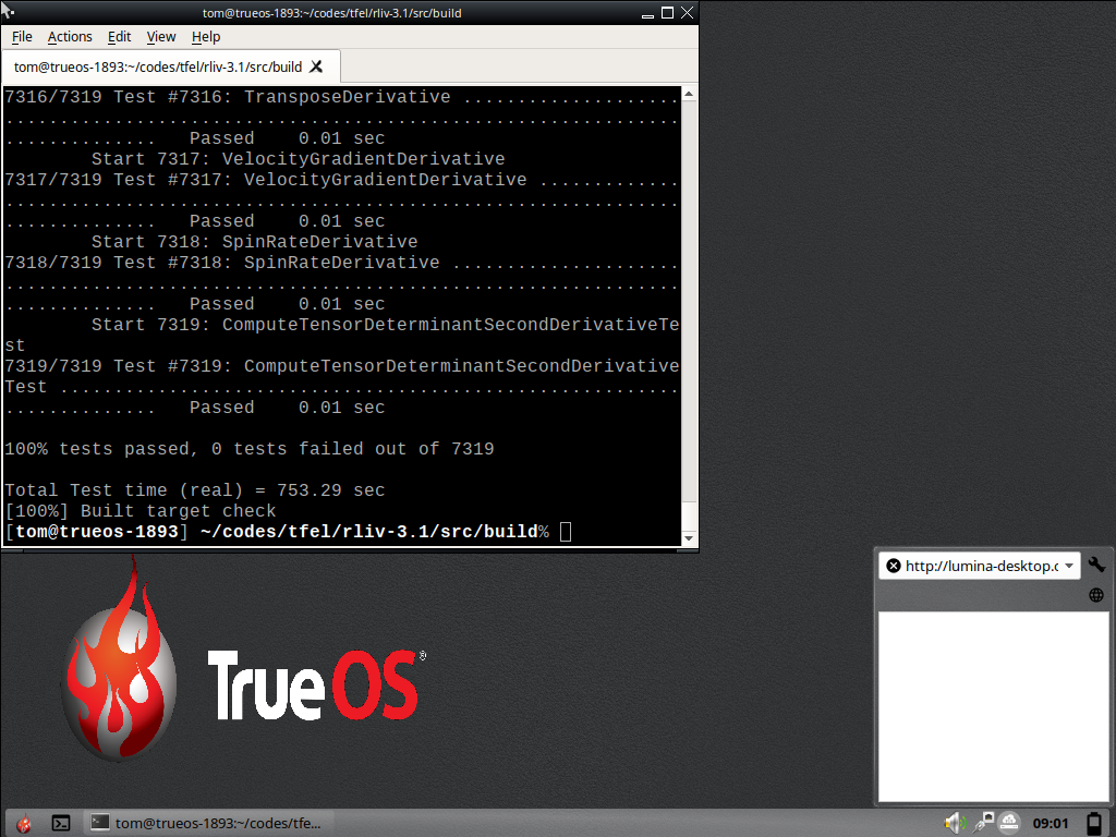
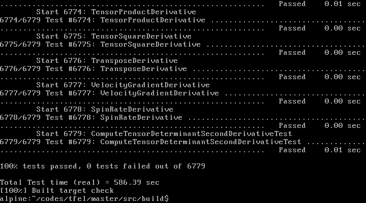
Portability is a convincing sign of software quality and maintainability:
C or C++
libraries.TFEL has been tested successfully on a various flavours
of LinuX and BSD systems (including
FreeBSD and OpenBSD). The first ones are
mostly built on gcc, libstdc++ and the
glibc. The second ones are built on clang and
libc++.
TFEL can be built on Windows in a wide
variety of configurations and compilers:
Visual Studio (2015
and 2017) or MingGW compilers.TFEL can be built in the Cygwin
environment.TFEL have reported to build successfully in the
Windows Subsystem for LinuX (WSL)
environment.
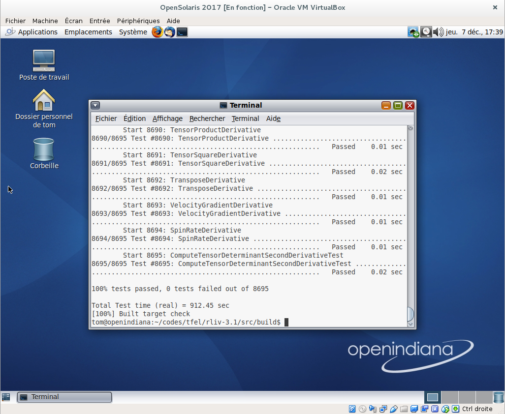
Although not officially supported, more exotic systems, such as
OpenSolaris and Haiku, have also been tested
successfully. The Minix operating systems provides a
pre-release of clang 3.4 that fails to compile
TFEL.
Version 3.1 has been tested using the following compilers:
gcc on various
POSIX systems: versions 4.7, 4.8, 4.9, 5.1, 5.2, 6.1, 6.2,
7.1, 7.2clang on various
POSIX systems: versions 3.5, 3.6, 3.7, 3.8, 3.9, 4.0,
5.0intel.
The only tested version is the 2018 version on LinuX. Intel compilers
15 and 16 are known not to work due to a bug in the EDG front-end that can’t parse a syntax
mandatory for the expression template engine. The same bug affects the
Blitz++ library
(see http://dsec.pku.edu.cn/~mendl/blitz/manual/blitz11.html).
Version 2017 shall work but were not tested.Visual Studio The
only supported versions are the 2015 and 2017 versions. Previous
versions do not provide a suitable C++11 support.PGI compiler (NVIDIA): version 17.10 on
LinuXMinGW has been tested successfully in a wide variety of
configurations/versions, including the version delivered with
Cast3M 2017.| Compiler and options | Success ratio | Test time |
|---|---|---|
gcc 4.9.2 |
100% tests passed | 681.19 sec |
gcc 4.9.2+fast-math |
100% tests passed | 572.48 sec |
clang 3.5 |
100% tests passed | 662.50 sec |
clang 3.5+libstcxx |
99% tests passed | 572.18 sec |
clang 5.0 |
100% tests passed | 662.50 sec |
icpc 2018 |
100% tests passed | 511.08 sec |
PGI 17.10 |
99% tests passed | 662.61 sec |
Concerning the PGI compilers, performances may be
affected by the fact that this compiler generates huge shared libraries
(three to ten times larger than other compilers).