This paper is dedicated to the implementation a perfect plastic behaviour based on the Hosford equivalent stress.

The whole implementation is available here.

Description

Elasticity

The elasticity is assumed linear and isotropic, i.e. given by the Hooke law: \[ \underline{\sigma}=\lambda\,{\mathrm{tr}{\left(\underline{\varepsilon}^{\mathrm{el}}\right)}}\,\underline{I}+2\,\mu\,\underline{\varepsilon}^{\mathrm{el}} \] where \(\lambda\) and \(\mu\) are the first and second Lamé parameters.

Plasticity

The yield surface is chosen as follows: \[ f{\left(\underline{\sigma}\right)}=\sigma_{\mathrm{eq}}^{H}-\sigma_{Y} \] where:

• \(\sigma_{\mathrm{eq}}^{H}\) is the Hosford equivalent stress defined hereafter.
• The yield stress \(\sigma_{Y}\) is a constant material parameter.

The Hosford equivalent stress is defined by (see [1]): \[ \sigma_{\mathrm{eq}}^{H}=\sqrt[a]{{{\displaystyle \frac{\displaystyle 1}{\displaystyle 2}}}{\left({\left|\sigma_{1}-\sigma_{2}\right|}^{a}+{\left|\sigma_{1}-\sigma_{3}\right|}^{a}+{\left|\sigma_{2}-\sigma_{3}\right|}^{a}\right)}} \] where \(\sigma_{1}\), \(\sigma_{2}\) and \(\sigma_{3}\) are the eigenvalues of the stress.

Therefore, when \(a\) goes to infinity, the Hosford stress reduces to the Tresca stress. When \(n = 2\) the Hosford stress reduces to the von Mises stress.

The Hosford stress is an isotropic homogeneous function of degree 1. The flow rule is assumed associated and the plastic strain rate \(\underline{\dot{\varepsilon}}^{\mathrm{p}}\) is given by: \[ \underline{\dot{\varepsilon}}^{\mathrm{p}}=\dot{p}\,{\displaystyle \frac{\displaystyle \partial \sigma_{\mathrm{eq}}^{H}}{\displaystyle \partial \underline{\sigma}}}=\dot{p}\,\underline{n}^{H} \] where \(\dot{p}\) is the rate of the equivalent plastic strain \(p\).

Implicit scheme

Choice of the state variables

The behaviour is integrated by an implicit scheme. Two state variables are introduced:

• the elastic strain \(\underline{\varepsilon}^{\mathrm{el}}\).
• the equivalent plastic strain \(p\).

The elastic strain is automatically defined by the Implicit domain specific language.

The latter could be considered as an integration variable, but, for post-processing purposes, we choose to keep it as a state variable.

Elastic prediction

First, an elastic prediction of the stress \(\underline{\sigma}^{\mathrm{tr}}\) is made (The following expression is not valid in plane stress hypothesis, see below): \[ \underline{\sigma}^{\mathrm{tr}}=\lambda\,{\mathrm{tr}{\left({\left.\underline{\varepsilon}^{\mathrm{el}}\right|_{t}}+\theta\,\Delta\,\underline{\varepsilon}^{\mathrm{to}}\right)}}\,\underline{I}+2\,\mu\,{\left({\left.\underline{\varepsilon}^{\mathrm{el}}\right|_{t}}+\theta\,\Delta\,\underline{\varepsilon}^{\mathrm{to}}\right)} \]

• If the predicted stress is inside the elastic domain, no plastic flow occurs.
• Otherwise, the material state at the end of the time step lies on the yield surface.

Equations governing the material evolution under plastic loading

The equation associated with the evolution of the elastic strain is given by the split of strain: \[ f_{\underline{\varepsilon}^{\mathrm{el}}}=\Delta\,\underline{\varepsilon}^{\mathrm{el}}-\Delta\,\underline{\varepsilon}^{\mathrm{to}}+\Delta\,p\,{\left.\underline{n}^{H}\right|_{t+\theta\,\Delta\,t}} \]

The derivatives of this equation with respect to \(\Delta\,\underline{\varepsilon}^{\mathrm{el}}\) and \(\Delta\,p\) are given by: \[ \left\{ \begin{aligned} {\displaystyle \frac{\displaystyle \partial f_{\underline{\varepsilon}^{\mathrm{el}}}}{\displaystyle \partial \Delta\,\underline{\varepsilon}^{\mathrm{el}}}} &= \underline{\underline{\mathbf{I}}}+2\,\mu\,\theta\,\Delta\,p\,{\displaystyle \frac{\displaystyle \partial {\left.\underline{n}^{H}\right|_{t+\theta\,\Delta\,t}}}{\displaystyle \partial {\left.\underline{\sigma}\right|_{t+\theta\,\Delta\,t}}}}\\ {\displaystyle \frac{\displaystyle \partial f_{\underline{\varepsilon}^{\mathrm{el}}}}{\displaystyle \partial \Delta\,\underline{\varepsilon}^{\mathrm{el}}}} &= {\left.\underline{n}^{H}\right|_{t+\theta\,\Delta\,t}}\\ \end{aligned} \right. \]

To determine the equivalent plastic strain increment, the following equation must be satisfied: \[ f_{p}={\left.\sigma_{\mathrm{eq}}^{H}\right|_{t+\theta\,\Delta\,t}}-\sigma_{Y}=0 \]

In the implementation described below, this equation will be normalised by the Young modulus to ensure that all equations have the same magnitude.

The derivatives of this equation with respect to \(\Delta\,\underline{\varepsilon}^{\mathrm{el}}\) and \(\Delta\,p\) are given by: \[ \left\{ \begin{aligned} {\displaystyle \frac{\displaystyle \partial f_{p}}{\displaystyle \partial \Delta\,\underline{\varepsilon}^{\mathrm{el}}}} &= 2\,\mu\,\theta\,{\left.\underline{n}^{H}\right|_{t+\theta\,\Delta\,t}}\\ {\displaystyle \frac{\displaystyle \partial f_{p}}{\displaystyle \partial \Delta\,p}} &= 0\\ \end{aligned} \right. \]

Implementation

Metadata

The beginning of the file gives some information about the behaviour:

• the integration scheme used, selected by the @DSL keyword.
• the name of the behaviour, introduced by the @Behaviour keyword.
• the author of the implementation (@Author).
• a small description of the behaviour (@Description).

@DSL       Implicit;
@Behaviour HosfordPerfectPlasticity;
@Author    Thomas Helfer;
@Description{
  A simple implementation of a perfect
  plasticity behaviour using the
  Hosford stress.
};

Supported modelling hypothesis

Thanks to the StandardElasticity brick, all the modelling hypotheses can be supported. The following statement, starting with the @ModellingHypotheses, enables all the modelling hypotheses:

@ModellingHypotheses {".+"};

The standard elasticity brick

To implement this behaviour, we will use the StandardElasticity brick which provides:

• Automatic computation of the stress tensor at various stages of the behaviour integration.
• Automatic computation of the consistent tangent operator.
• Automatic support for plane stress and generalized plane stress modelling hypotheses (The axial strain is defined as an additional state variable and the associated equation in the implicit system is added to enforce the plane stess condition).
• Automatic addition of the standard terms associated with the elastic strain state variable.

This behaviour brick is fully described here.

The usage of the StandardElasticity is introduced as follows:

@Brick StandardElasticity;

Numerical parameters

The following part of file give some default values for numerical parameters used by the integration algorithm:

@Epsilon 1.e-16;
@Theta 1;

State variables

The elastic strain is automatically declared the StandardElasticity brick. The associated variable is eel.

The following statement introduces the equivalent plastic strain named p:

@StateVariable strain p;
p.setGlossaryName("EquivalentPlasticStrain");

Material constants

The material properties are hard-coded. The @ElasticMaterialProperties is used to declare the Young modulus and the Poisson ratio.

@ElasticMaterialProperties {150e9,0.3};

In the Implicit scheme, the lame coefficients are automatically deduced from the Young modulus and the Poisson ratio. They are accessible though the lambda and mu local variables which are automatically defined.

The parameters associated with the plastic part of the behaviour are defined as follows:

@Parameter a    = 8;
@Parameter sigy = 150e6;

Here a stands for the Hosford exponent and sigy is the yield stress.

Local variable declaration

A boolean b is declared as a local variable.

@LocalVariable bool b;

This boolean will be true if plastic loading occurs.

Local variable initialization

The main goal of the local variable initialization is to test if the elastic prediction of the stress lies inside the yield surface.

@InitializeLocalVariables{
  const stress seps = 1.e-10*young;
  const auto sigel = computeElasticPrediction();
  const auto seqel = computeHosfordStress(sigel,a,seps);
  b = seqel>sigy;
}

The computeElasticPrediction method, provided by the StandardElasticity brick, computes the elastic prediction of the stress and takes into account the modelling hypothesis. This prediction is thus valid under the plane stress hypothesis.

The computeHosfordStress is then called. It takes three arguments:

• the stress,
• the Hosford exponent,
• a criterion used to check if the von Mises stress is non zero. The von Mises stress is used to normalize the eigenvalues of the stress and avoid numerical overflows (See [2] for details).

At the last line, the boolean variable b is set to true if the elastic prediction of the Hosford stress exceeds the yield stress.

Implicit system

The code describing the implicit system is rather short:

@Integrator{
  const stress seps = 1.e-10*young;
  if(!b){
    // elastic loading, nothing to be done
    return true;
  }
  real seq;
  Stensor n;
  Stensor4 dn;
  std::tie(seq,n,dn) = computeHosfordStressSecondDerivative(sig,a,seps);
  feel        += dp*n;
  dfeel_ddeel += 2*mu*theta*dp*dn;
  dfeel_ddp    = n;
  fp           = (seq-sigy)/young;
  dfp_ddeel    = 2*mu*theta*n/young;
  // this is a small trick that is necessary if the first time
  // step leads to a plastic loading:
  // on this case, the stress are zero on the first iteration and
  // this results in a null line in the jacobian matrix because
  // the normal is then undefined.
  // To avoid the issue, we arbitrarily set dfp_ddp to 1 in that case. 
  dfp_ddp      = (seq<seps) ? 1:  0;
}

It shall be noted that, at the beginning of this code block:

• feel has been initialized to \(\Delta\,\underline{\varepsilon}^{\mathrm{el}}-\Delta\,\underline{\varepsilon}^{\mathrm{to}}\) by the StandardElasticity brick
• fp has been initialized to \(\Delta\,p\) following standard conventions defined in the the Implicit domain specific language.
• the jacobian has been set to identity, following standard conventions defined in the Implicit domain specific language.

Thus, all the variables have been set to describe a purely elastic behaviour. Hence, nothing is to be done if the boolean variable b is false. In this case, one just return true.

If a plastic loading has been predicted, one uses the computeHosfordStressSecondDerivative function which returns:

• the Hosford stress seq
• the Hosford stress derivative n with respect to the stress
• the Hosford stress second derivative dn with respect to the stress

The implicit system is then readily written, using expressions given in the previous paragraph.

Note With C++-17 structured bindings enabled, the previous code is much more readable:

@Integrator{
  const stress seps = 1.e-10*young;
  if(!b){
    // elastic loading, nothing to be done
    return true;
  }
  const auto [seq,n,dn] = computeHosfordStressSecondDerivative(sig,a,seps);
  feel        += dp*n;
  dfeel_ddeel += 2*mu*theta*dp*dn;
  dfeel_ddp    = n;
  fp           = (seq-sigy)/young;
  dfp_ddeel    = 2*mu*theta*n/young;
  dfp_ddp      = 0;
}

Determining the yield surface in plane stress

In this section, we show how to use a simple python script to determine the yield surface in plane stress.

Compilation of the behaviour

$ mfront --obuild --interface=abaqus HosfordPerfectPlasticity.mfront
Treating target : all
The following library has been built :
- libABAQUSBEHAVIOUR.so :  HOSFORDPERFECTPLASTICITY_AXIS HOSFORDPERFECTPLASTICITY_PSTRESS HOSFORDPERFECTPLASTICITY_PSTRAIN HOSFORDPERFECTPLASTICITY_3D

A simple python script to determine the yield surface in plane stress

The following script determines the yield stress under the plane stress assumption in the principal stress space by a brute force approach. It imposes strain paths in varying directions and a constraint the shear stress is null. The computations stops when the plastic equivalent strain exceeds \(10^{-3}\). The current stress state is then printed.

from math import pi,cos,sin,sqrt
import mtest

for theta in [pi*(-1+2*float(i)/99) for i in range(0,100)]:
    em   = 2.e-2
    npas = 100
    tmax = 1
    c    = cos(theta)
    s    = sin(theta)
    m    = mtest.MTest()
    mtest.setVerboseMode(mtest.VerboseLevel.VERBOSE_QUIET)
    m.setModellingHypothesis('PlaneStress')
    m.setMaximumNumberOfSubSteps(1)
    m.setBehaviour('abaqus','src/libABAQUSBEHAVIOUR.so',
                   'HOSFORDPERFECTPLASTICITY_PSTRESS');
    m.setExternalStateVariable("Temperature",293.15)
    m.setImposedStrain('EXX',{0:0,tmax:em*c})
    m.setImposedStrain('EYY',{0:0,tmax:em*s})
    m.setNonLinearConstraint('SXY','Stress')
    s  = mtest.MTestCurrentState()
    wk = mtest.MTestWorkSpace()    
    m.completeInitialisation()    
    m.initializeCurrentState(s)
    m.initializeWorkSpace(wk)
    ltime=[(tmax/(npas-1))*i for i in range(npas)]
    for i in range(npas-1):
        m.execute(s,wk,ltime[i],ltime[i+1])
        p = s.getInternalStateVariableValue('EquivalentPlasticStrain');
        if(p>0.001):
            print(str(theta)+" "+str(s.s1[0])+" "+str(s.s1[1]))
            break

Comparing the robustness of various algorithms

This section compares the robustness of various algorithms used to solve the implicit system used to integrate the Hosford behaviour.

Description of the test

The test presented is based on the paper of Scherzinger (see [2]). The test is based on the following steps:

• A direction in the \(\pi\)-plane, characterized by an angle \(\alpha\), is choosen. \(\alpha\) varies from \(-\pi\) to \(\pi\): this range is discretized \(1000\) times.
• A stress state \(\underline{\sigma}_{\alpha}\) which lies on the yield surface \(\sigma_{\mathrm{eq}}^{H}=\sigma_{Y}\) is determined. Such a stress state is characterized by its unique coordinates \(\tilde{\pi}{\left(\underline{\sigma}_{\alpha}\right)}\) in the \(\pi\)-plane and this projection determines its three eigenvalues. \(\underline{\sigma}_{\alpha}\) is choosen diagonal.
• The elastic strain \(\underline{\varepsilon}^{\mathrm{el}}_{\alpha}\) corresponding to \(\underline{\sigma}_{\alpha}\) is determined.
• Starting from a virgin state (all state variables are set to zero), the behaviour is integrated multiple times by imposing a strain increment \(\Delta\,\underline{\varepsilon}^{\mathrm{to}}\) equal to \(x\,\underline{\varepsilon}^{\mathrm{el}}_{\alpha}\) where \(x\) is increased from \(1\) to a maximal value of \(30\). If the behaviour integration succeeds, \(x\) is increased by an increment egal to \(30/1000\). This step is stopped if the behaviour integration fails or if \(x\) reaches \(30\).

For each values of \(\alpha\) and \(x\), the number of iterations needed to solve the implicit system is recorded.

The implementation presented so far is modified to declare an additional state variable using to save the number of iterations required to reach the convergence.

The python script which implements the test is the following, in the case of a Hosford exponent egal to \(100\):

from math import pi,cos,sin
import tfel.math     as tmath
import tfel.material as tmaterial
import mtest

nmax  = 1000
nmax2 = 1000
E  = 150e9
nu = 0.3
s0 = 150e6

for a in [pi*(-1.+(2.*i)/(nmax-1)) for i in range(0,nmax)]:
    for x in [1+(29.*i)/(nmax2-1)  for i in range(0,nmax2)]:
        nbiter=0
        s     = tmath.makeStensor3D(tmaterial.buildFromPiPlane(cos(a),sin(a)))
        seq   = tmaterial.computeHosfordStress(s,100,1.e-12);
        s    *= x*(s0/seq)
        e0    = (s[0]-nu*(s[1]+s[2]))/E
        e1    = (s[1]-nu*(s[0]+s[2]))/E
        e2    = (s[2]-nu*(s[0]+s[1]))/E
        m    = mtest.MTest()
        mtest.setVerboseMode(mtest.VerboseLevel.VERBOSE_QUIET)
        m.setModellingHypothesis('Tridimensional')
        m.setMaximumNumberOfSubSteps(1)
        m.setBehaviour('abaqus','src/libABAQUSBEHAVIOUR.so',
                       'HOSFORDPERFECTPLASTICITY100_3D');
        m.setExternalStateVariable("Temperature",293.15)
        m.setImposedStrain('EXX',{0:0,1:e0})
        m.setImposedStrain('EYY',{0:0,1:e1})
        m.setImposedStrain('EZZ',{0:0,1:e2})
        m.setImposedStrain('EXY',0)
        m.setImposedStrain('EXZ',0)
        m.setImposedStrain('EYZ',0)
        s  = mtest.MTestCurrentState()
        wk = mtest.MTestWorkSpace()
        m.completeInitialisation()
        m.initializeCurrentState(s)
        m.initializeWorkSpace(wk)
        try:
            m.execute(s,wk,0,1)
            nbiter=s.getInternalStateVariableValue("NumberOfIterations")
        except:
            nbiter=100
            break
        print(str((x/seq)*cos(a))+" "+str((x/seq)*sin(a))+" "+str(nbiter))
    print()

This script outputs, for each couple \({\left(\alpha,x\right)}\) for which the behaviour integration succeeds, the coordinates \(\tilde{\pi}{\left(\underline{\sigma}_{\alpha}\right)}\) scaled by \(\sigma_{Y}\) and the number of iterations required to reach the convergence.

Algorithms tested

The following algorithms are considered:

• Algorithm 1: The standard Newton-Raphson algorithm.
• Algorithm 2: The Newton-Raphson algorithm with a test on the value of the equivalent Hosford stress \({\left.\sigma_{\mathrm{eq}}^{H}\right|_{t+\theta\,\Delta\,t}}\) for the current estimation of the elastic strain increment. If this \({\left.\sigma_{\mathrm{eq}}^{H}\right|_{t+\theta\,\Delta\,t}}\) is greater than \(\beta\,\sigma_{Y}\), the Newton step is rejected: the direction is kept unchanged but the amplitude of the correction to the internal state variables increment is divided by two. In the following, \(\beta\) is choosen equal to \(\frac{3}{2}\). The test has to be made in the @Integrator code block: if the test fails, one just have to return the false value. This is obtained by adding the following line after the computation of the Hosford equivalent stress:

if(seq>3*(sigy/2)){
  return false;
}

• Algorithm 3: The Newton-Raphson algorithm with a limitation of the increment of the elastic strain increment at each iteration. This can be activated by using the setMaximumIncrementValuePerIteration method on the eel variable.
• Algorithm 4: The standard Levenberg-Marquardt algorithm. This algorithm is selected using the @Algorithm keyword.

Hosford \(a=6\)

The Hosford yield surface for an exponent egal to \(a=6\) is smooth.

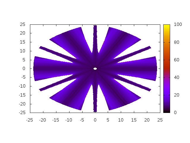
Figure 1 displays the output of the previous script in the \(\pi\)-plane (each coordinate being scaled by \(\sigma_{Y}\)). The maximum number of iteration allowed to reach the convergence is \(100\) by default. However, as stated by Scherzinger, if the convergence is not reached for \(30\) iterations, most of the time the convergence will not be reached.

The results depicted on Figure 1 confirms the ones of Scherzinger: the standard Newton algorithm conditionally converges. Indeed, it can be seen that the standard Newton algorithm converges for all values of \(\alpha\) if \(x\) is low enough. For large values of \(x\), the convergence clearly depends on \(\alpha\).

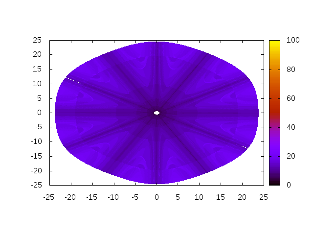
Figure 2 displays the output of the previous script for the second algorithm. This figure shows that this slight modification of the standard Newton algorithm considerably increases the robustness: the convergence is reached for all tested values of \(\alpha\) and \(x\).

Results for the third and fourth algorithms are not shown but are very similar to the one obtained with the second algorithm. Indeed, in terms of robustness, differences between those three algorithms only arises for high values of the Hosford exponent \(a\).

Hosford \(a=8\)

For an exponent equal to \(a=8\), the curvature of the yield surface varies more rapidly.

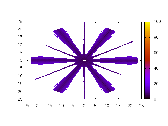
As already stated by Scherzinger, Figure 3 shows that the performance in terms of robustness of the standard Newton algorithm is getting worse as the Hosford exponent increases.

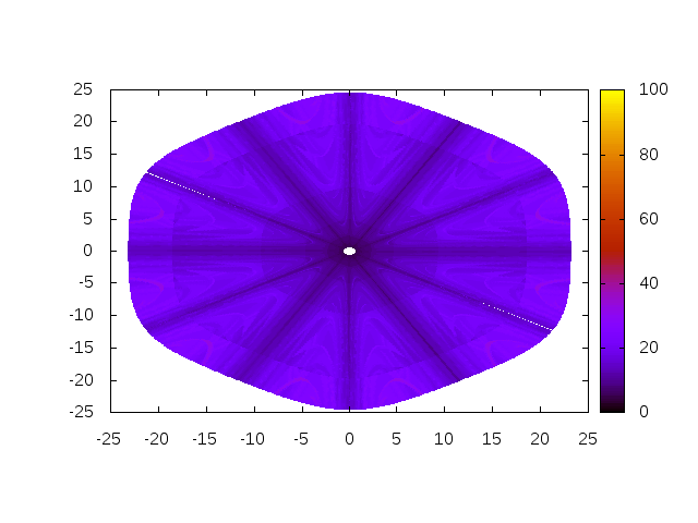
Again, Algorithm 2 shows a remarkable benefit in terms of robustness.

Hosford \(a=100\)

For a very high exponent \(a=100\), the yield surface is very close to the Tresca yield surface and shows very sharp edges.

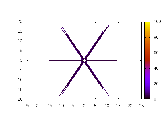
Figure 5 shows that the standard Newton algorithm performs very poorly.

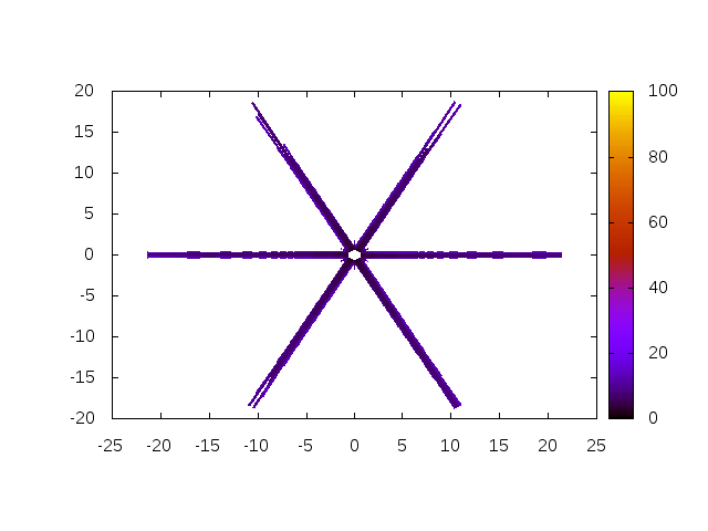
In this case, the second algorithm does not improve the robustness as shown on Figure 6. This algorithm performs almost as poorly than the standard Newton algorithm.

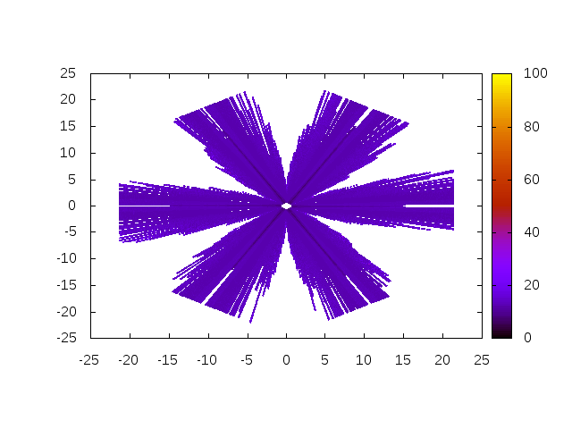
Figure 7 shows that the third algorithm clearly increases the robustness in some directions but the robustness remains low for angles close the edges of the yield surfaces.

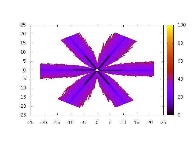
Figure 7 shows that the Levenberg-Marquardt algorithm outperforms Algorithm 3. However, the robustness remains low for angles close the edges of the yield surfaces.

Influence of the eigen solver

In this section, we consider the influence of the eigen solver. In the previous tests, the default eigen solver was used. This analytical solver has been shown to provide a very interesting trade-off between accuracy and numerical efficiency. It was also shown that the Jacobi eigensolver provides very accurate results but is less efficient by our default eigen solver (about 2 times less efficient).

Our tests, not reported here, shows that changing the eigen solver:

• does not change the results presented for exponents \(a=6\) and \(a=8\).
• does not increase the robustness of the first and second algorithms for \(a=100\).

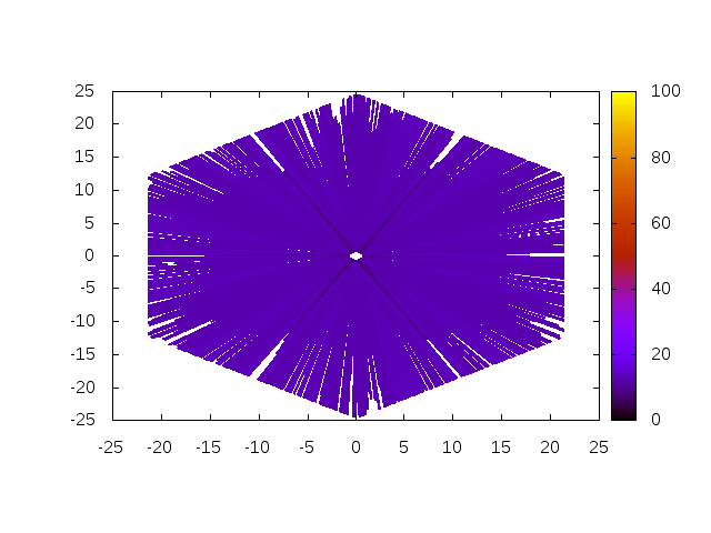
Figure 9 shows that using the Jacobi eigen solver has a strong influence on the robustness of Algorithm 3.

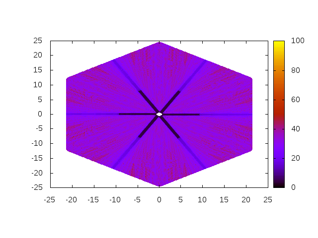
Using the Jacobi eigen solver with Algorithm 4 shows that convergence is reached for all tested values of \(\alpha\) and \(x\).

Conclusions

Our tests shows that for high values of the Hosford exponent, sophisticated algorithms and accurate eigen solvers are required to guarantee the convergence of the algorithm for large trial stress.

However, for standard values of the Hosford exponent (\(a=6\) and \(a=8\)), our results shows that Algorithm 2, which a very simple modification of the standard Newton algorithm based on a simple and intuitive physical consideration, is very robust.

Those results has to confirmed on real structural analyses. In particular, the impact of each algorithms on the overall efficiency of the simulations has to be evaluated.

References