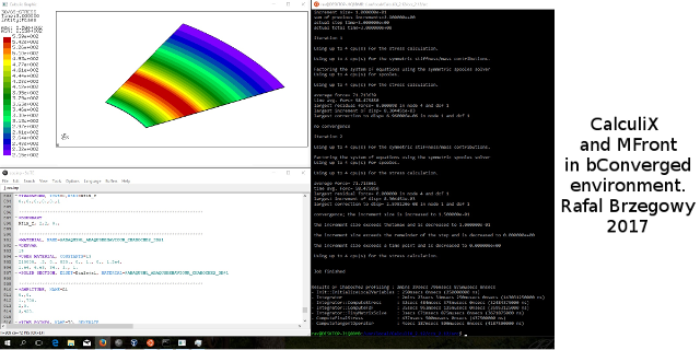
User defined behaviour in `CalculiX`

User-defined mechanical behavior can be implemented using three different interfaces:

The native CalculiX interface.
The ABAQUS umat routines for linear materials (small strain analyses).
The ABAQUSNL umat routines for non-linear materials (finite strain analyses).

There are two ways of introducing user-defined mechanical behavior:

Modify the CalculiX sources. This option is supported for the three interfaces.
Call a behavior defined in shared libraries.

Each of these approaches has its own advantages and its own pitfalls.

The first one is intrusive and requires a partial recompilation of CalculiX, which means having access to the sources and the rights to install the executable if it is meant to be deployed on a system-wide location.

The second one does not require any modification to CalculiX, is generally easier to set up and is very flexible. There is no intrinsic limitations on the number of shared libraries and functions that can be dynamically loaded. It is thus quite feasible to create mechanical behaviours databases by creating a shared library by specific material. Such libraries will only be loaded if needed. In such an approach, the mechanical behaviour is dedicated to a specific material and is self-contained: it has no external parameter.

Shared libraries can be shared between co-workers by moving them on a shared folder.

However, experience shows that using shared libraries can be confusing for some user as they have to update their environment variables (PATH on Windows or LD_LIBRARY_PATH on Unixes) for the libraries to be usable. Shared libraries can also be more sensible to system updates.

Note

Calling external libraries from CalculiX for the ABAQUS and ABAQUSNL is supported in CalculiX since version 2.12. If you are compiling CalculiX from the sources, you must use the Makefile_MFront file (which is part from the sources) to enable it.

Calling external libraries from CalculiX for the native interface requires a patch in version 2.12 that can be downloaded here.

Using the `CalculiX` native interface

When compiling a MFront behaviour, the CalculiX native interface is invoked as follows:

$ mfront --obuild --interface=calculix Chaboche.mfront
Treating target : all
The following library has been built :
- libCALCULIXBEHAVIOUR.so :  CHABOCHE

The libCALCULIXBEHAVIOUR.so is generated in the src subdirectory. This library shall be copied in a location where the dynamic load can find it. Another solution is to add the src directory to the LD_LIBRARY_PATH as follows:

$ export LD_LIBRARY_PATH=$(pwd)/src:$LD_LIBRARY_PATH

A template for the behaviour declaration has been generated in the calculix subdirectory.

** 
** File generated by MFront from the Chaboche.mfront source
** Example of how to use the Chaboche behaviour law
** Author Jean - Michel Proix
** Date   26 / 11 / 2013
**

*Material, name=@CALCULIXBEHAVIOUR_CHABOCHE
*Depvar
19
** The material properties are given as if we used parameters to explicitly
** display their names. Users shall replace those declaration by
** theirs values
*User Material, constants=12
<YoungModulus>, <PoissonRatio>, <R_inf>, <R_0>, <b>, <k>, <w>, <C_inf_0>, 
<C_inf_1>, <g_0_0>, <g_0_1>, <a_inf>

The interesting part here is the name of the material: CALCULIXBEHAVIOUR_CHABOCHE, which can be decomposed in two parts separated by the underscore character (_):

The first part, CALCULIXBEHAVIOUR, is used to determine in which library the external function is implemented.
The second part, CHABOCHE, gives the name of external function to be called.

Here, the library name has been stripped from system-specific convention (the leading lib and the .so extension). The base name of the library and the name of the function must be upper-cased. This is due to the way CalculiX interprets the input file.

The material name can optionally end with an identifier beginning by the @ character. This character can be followed by any character and is used to declare two distinct materials based on the same external behaviour having different material coefficients. For example, the following example declares two distinct materials relying on the same external behaviour:

*Material, name=@CALCULIXBEHAVIOUR_ELASTICITY@1
** The material properties are given as if we used parameters to explicitly
** display their names. Users shall replace those declaration by
** theirs values
*User Material, constants=2
150000,0.3

*Material, name=@CALCULIXBEHAVIOUR_ELASTICITY@2
*User Material, constants=2
200000,0.3

Using a small strain behaviour in finite strain analysis

In finite strain, CalculiX replaces the linearised strain by the Green-Lagrange strain and interprets the output of the behaviour as the second Piola-Kirchhoff stress. This allows small strain behaviours to be used in the context of finite rotations and this procedure is equivalent to the FiniteRotationSmallStrain introduced by MFront in most interfaces. However, this procedure is said to be limited to small strain because the trace of the Green-Lagrange strain is not related to the change of volume, which is basis of most behaviours describing plasticity and viscoplasticity in small strain: indeed, even though the plastic strain is traceless, the plastic flow will not be isochoric.

The situation is quite different in the ABAQUSNL interface where the Hencky strain (logarithmic strain) is used (see below): the trace of the logarithmic strain is directly linked to the change of volume.

This situation is also different from the strategy used in Abaqus/Standard which tries to integrate the behaviour in rate form and then uses the Jauman objective stress rate to ensure objectivity (see [1]): this approach is based of the fact that the trace of the deformation rate is directly linked to the change of volume.

To describe plasticity and viscoplasticity at finite strain using an additive decomposition of the strain, we recommend using the ‘MieheApelLambrechtLogarithmicStrain’ finite strain strategy in MFront which is also based on the Hencky strain but interprets the output of the behaviour as the dual of the Hencky strain, which is consistent from the point of view of energy and automatically ensures objectivity. See [2] for details.

Using the `Abaqus/Standard` interface

For performance reasons, CalculiX supports two kinds of interfaces to Abaqus/Standard’s umat behaviours:

ABAQUS is meant to describe linear materials.
ABAQUSNL is meant to describe no linear materials. For nonlinear materials the logarithmic strain and infinitesimal rotation are calculated, which slows down the calculation. Consequently, the nonlinear routine should only be used if necessary.

Those two interface supports the call to behaviours in external shared libraries.

Calling shared libraries is triggered by putting the @ character in front material name. The material name is then decomposed into three parts, separated by the _ character:

The name of the interface (ABAQUS or ABAQUSNL).
The base name of the shared library (see below).
The name of the function implementing the behavior.

For instance, if we want to call a small strain behavior in a linear analysis, implemented by the CHABOCHE function in the libABAQUSBEHAVIOURS.so shared library (Under Windows, the library name has the dll extension.), one would declare the following material name:

@ABAQUS_ABAQUSBEHAVIOURS_CHABOCHE

Using the `MFront` behaviours generated through the `abaqus` interface

As described in the previous section, calling shared libraries in only supported for the ABAQUS or ABAQUSNL interfaces. This means that we can call mechanical behaviours generated by MFront through the abaqus interface quite easily.

The abaqus interface is described here.

A first example, the Saint-Venant Kirchoff hyperelastic behaviour

Generation of the shared library

Consider the Saint-Venant Kirchoff hyperelastic behaviour as implemented here.

The library is generated like this:

$ mfront --obuild --interface=abaqus SaintVenantKirchhoffElasticity.mfront 
Treating target : all
The following library has been built :
- libABAQUSBEHAVIOUR.so :  SAINTVENANTKIRCHHOFFELASTICITY_AXIS SAINTVENANTKIRCHHOFFELASTICITY_PSTRAIN SAINTVENANTKIRCHHOFFELASTICITY_3D

This shows that the library libABAQUSBEHAVIOUR.so has been generated. Then, we have one implementation per modelling hypothesis. For a $3D$ computation, one shall use the SAINTVENANTKIRCHHOFFELASTICITY_3D function.

Thus, the material name to be used is: @ABAQUSNL_ABAQUSBEHAVIOUR_SAINTVENANTKIRCHHOFFELASTICITY_3D.

Known issue with CalculiX 2.12

The source code generated by MFront contains a test that checks if the behaviour is called in a finite strain resolution. This information is not available in CalculiX 2.12, so the generation of the library must be made as follows:

Generate the sources:
$ mfront --interface=abaqus SaintVenantKirchhoffElasticity.mfront
Modify the sources:

Comment all the blocks in the src/abaqusSaintVenantKirchhoffElasticity.cxx file of the form:
if(KSTEP[2]!=1){
std::cerr << "the SaintVenantKirchhoffElasticity behaviour is only valid in finite strain analysis\n";
*PNEWDT=-1;
return;
}
Compile the library:
$ mfront --obuild

Another solution is to deactive checks (for TFEL greater than 3.1) like this:
$ mfront --obuild -D MFRONT_ABAQUS_NORUNTIMECHECKS --interface=abaqus SaintVenantKirchhoffElasticity.mfront

A simple tensile test

The description of a simple tensile test is as follows:

**
** GEOMETRY
**
*Node
      1,           0.,         0.,         1.
      2,           0.,         1.,         1.
      3,           0.,         0.,         0.
      4,           0.,         1.,         0.
      5,           1.,         0.,         1.
      6,           1.,         1.,         1.
      7,           1.,         0.,         0.
      8,           1.,         1.,         0.
*Element, type=C3D8, elset=cube
1, 5, 6, 8, 7, 1, 2, 4, 3
*Solid Section, elset=cube, material=@ABAQUSNL_ABAQUSBEHAVIOUR_SAINTVENANTKIRCHHOFFELASTICITY_3D
,
*Nset, nset=sx2, generate
 5,  8,  1
*Nset, nset=sx1, generate
 1,  4,  1
*Nset, nset=sy1
 1,  3,  5,  7
*Nset, nset=sy2
 2,  4,  6,  8,
*Nset, nset=sz1
 3,  4,  7,  8
*Nset, nset=sz2
 1,  2,  5,  6,
**
** MATERIAL
** 
*Material, name=@ABAQUSNL_AbaqusBehaviour_SaintVenantKirchhoffElasticity_3D
*Depvar
   0
* User Material, constants=2
  150e9, 0.34
**
** LOADING
** 
*Step, nlgeom=YES
*Static
0.02, 1., 1e-05, 0.2
*Boundary
sx1, 1, 1
*Boundary
sy1, 2,2
*Boundary
sz1, 3,3
*Boundary
sx2, 1, 1, 0.2
*EL PRINT, ELSET=cube
E, S
*End Step

Named state variables

MFront generates an example showing how to use the behaviour in Abaqus/Standard. Such example names each state variables, which is useful for post-processing. However, this feature is currently not supported by CalculiX.

Known issues

`ABAQUS` and `ABAQUSNL` interfaces

Number of states variables and number of material properties

In CalculiX 2.12, the value of the NSTATV argument passed to the ABAQUS and ABAQUSNL interfaces is the maximum number of state variables for all the materials. This is not what consistent with Abaqus/Standard which passes the number of state variables of the material.

The same remarks applies to the number of the material properties (NPROPS argument).

This issue can be circumvented by disabling checks in MFront:

$ mfront --obuild -D MFRONT_ABAQUS_NORUNTIMECHECKS --interface=abaqus SaintVenantKirchhoffElasticity.mfront

Behaviours at finite strain with `CalculiX` 2.12

The source code generated by MFront contains a test that checks if the behaviour is called in a finite strain resolution. This information is not available in CalculiX 2.12. See the SaintVenantKirchhoffElasticity example for details of how to circumvent this issue.

Benchmarks

Small strain

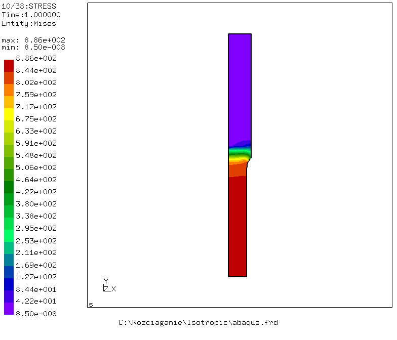
This example describes a tensile test on an AE specimen using an isotropic linear hardening plasticity behaviour depicted on the previous figure.

CPU times between the native implementation and the MFront implementation (using the CalculiX interface) are reported in the following table:

	`CalculiX`	`MFront`
real	7m43.588s	8m6.849s
user	7m40.572s	7m59.904s
sys	0m4.180s	0m6.676s

Those figures show that using the MFront implementation is $4.9\%$ slower. Using the callgrind profiling tool of valgrind framework, one can see that more time is spent in looking for function calculix_searchExternalBehaviours than in the behaviour integration: $2.65\%$ of the time vs $1.66\%$ !

This is du to the mostly non-intrusive way of introducing external behaviours in CalculiX. This additional cost could totally disappear with a more clever and intrusive development.

If those 2.65% are removed from the total computational time, the MFront only causes to a $2.3\%$ slow down, which is acceptable.

This slow down could be du to the fact that the MFront behaviours update the elastic strain and recomputes the stress (it does not simply update it by adding an increment, as this is done in most implementation). Using the elastic strain is mandatory to handle properly material properties changing with temperature and thermal expansion.

References

Hughes, Thomas J. R. and Winget, James. Finite rotation effects in numerical integration of rate constitutive equations arising in large-deformation analysis. International Journal for Numerical Methods in Engineering. 1980. Vol. 15, no. 12, p. 1862–1867. DOI 10.1002/nme.1620151210. Available from: http://dx.doi.org/10.1002/nme.1620151210

Miehe, C., Apel, N. and Lambrecht, M. Anisotropic additive plasticity in the logarithmic strain space: Modular kinematic formulation and implementation based on incremental minimization principles for standard materials. Computer Methods in Applied Mechanics and Engineering. November 2002. Vol. 191, no. 47–48, p. 5383–5425. DOI 10.1016/S0045-7825(02)00438-3. Available from: http://www.sciencedirect.com/science/article/pii/S0045782502004383

How to use `MFront` in `CalculiX`

Thomas Helfer, Rafal Brzegowy

2/02/2017

User defined behaviour in `CalculiX`

Using the `CalculiX` native interface

Using a small strain behaviour in finite strain analysis

Using the `Abaqus/Standard` interface

Using the `MFront` behaviours generated through the `abaqus` interface

A first example, the Saint-Venant Kirchoff hyperelastic behaviour

Generation of the shared library

A simple tensile test

Known issues

`ABAQUS` and `ABAQUSNL` interfaces

Number of states variables and number of material properties

Behaviours at finite strain with `CalculiX` 2.12

Benchmarks

Small strain

References

How to use MFront in CalculiX

Thomas Helfer, Rafal Brzegowy

2/02/2017

User defined behaviour in CalculiX

Using the CalculiX native interface

Using a small strain behaviour in finite strain analysis

Using the Abaqus/Standard interface

Using the MFront behaviours generated through the abaqus interface

A first example, the Saint-Venant Kirchoff hyperelastic behaviour

Generation of the shared library

A simple tensile test

Known issues

ABAQUS and ABAQUSNL interfaces

Number of states variables and number of material properties

Behaviours at finite strain with CalculiX 2.12

Benchmarks

Small strain

References

How to use `MFront` in `CalculiX`

User defined behaviour in `CalculiX`

Using the `CalculiX` native interface

Using the `Abaqus/Standard` interface

Using the `MFront` behaviours generated through the `abaqus` interface

`ABAQUS` and `ABAQUSNL` interfaces

Behaviours at finite strain with `CalculiX` 2.12