
The header TFEL/Material/Hosford1972YieldCriterion.hxx
introduces three functions which are meant to compute the Hosford
equivalent stress and its first and second derivatives. This header
is automatically included by MFront
The Hosford equivalent stress is defined by: \[ \sigma_{\mathrm{eq}}^{H}=\sqrt[a]{\displaystyle\frac{\displaystyle 1}{\displaystyle 2}\left({\left|\sigma_{1}-\sigma_{2}\right|}^{a}+{\left|\sigma_{1}-\sigma_{3}\right|}^{a}+{\left|\sigma_{2}-\sigma_{3}\right|}^{a}\right)} \] where \(s_{1}\), \(s_{2}\) and \(s_{3}\) are the eigenvalues of the stress.
Therefore, when \(a\) goes to infinity, the Hosford stress reduces to the Tresca stress. When \(n = 2\) the Hosford stress reduces to the von Mises stress.
The following functions have been implemented:
computeHosfordStress: return the Hosford equivalent
stresscomputeHosfordStressNormal: return a tuple containing
the Hosford equivalent stress and its first derivative (the normal)computeHosfordStressSecondDerivative: return a tuple
containing the Hosford equivalent stress, its first derivative (the
normal) and the second derivative.The following example computes the Hosford equivalent stress, its normal and second derivative:
stress seq;
Stensor  n;
Stensor4 dn;
std::tie(seq,n,dn) = computeHosfordStressSecondDerivative(s,a,seps);
In this example, s is the stress tensor, a
is the Hosford exponent, seps is a numerical parameter used
to detect when two eigenvalues are equal.
If C++-17 is available, the previous code can be made
much more readable:
const auto [seq,n,dn] = computeHosfordStressSecondDerivative(s,a,seps);The header TFEL/Material/Barlat2004YieldCriterion.hxx
introduces various functions which are meant to compute the Barlat
equivalent stress and its first and second derivatives. This header
is automatically included by MFront for orthotropic
behaviours.
The Barlat equivalent stress is defined as follows (see [1]): \[ \sigma_{\mathrm{eq}}^{B}= \sqrt[a]{ \frac{1}{4}\left( \sum_{i=0}^{3} \sum_{j=0}^{3} {\left|s'_{i}-s''_{j}\right|}^{a} \right) } \]
where \(s'_{i}\) and \(s''_{i}\) are the eigenvalues of two transformed stresses \(\underline{s}'\) and \(\underline{s}''\) by two linear transformations \(\underline{\underline{\mathbf{L}}}'\) and \(\underline{\underline{\mathbf{L}}}''\): \[ \left\{ \begin{aligned} \underline{s}' &= \underline{\underline{\mathbf{L'}}} \,\colon\,\underline{\sigma}\\ \underline{s}'' &= \underline{\underline{\mathbf{L''}}}\,\colon\,\underline{\sigma}\\ \end{aligned} \right. \]
The linear transformations \(\underline{\underline{\mathbf{L}}}'\) and \(\underline{\underline{\mathbf{L}}}''\) are defined by \(9\) coefficients (each) which describe the material orthotropy. They are defined through auxiliary linear transformations \(\underline{\underline{\mathbf{C}}}'\) and \(\underline{\underline{\mathbf{C}}}''\) as follows: \[ \begin{aligned} \underline{\underline{\mathbf{L}}}' &=\underline{\underline{\mathbf{C}}}'\,\colon\,\underline{\underline{\mathbf{M}}} \\ \underline{\underline{\mathbf{L}}}''&=\underline{\underline{\mathbf{C}}}''\,\colon\,\underline{\underline{\mathbf{M}}} \end{aligned} \] where \(\underline{\underline{\mathbf{M}}}\) is the transformation of the stress to its deviator: \[ \underline{\underline{\mathbf{M}}}=\underline{\underline{\mathbf{I}}}-\displaystyle\frac{\displaystyle 1}{\displaystyle 3}\underline{I}\,\otimes\,\underline{I} \]
The linear transformations \(\underline{\underline{\mathbf{C}}}'\) and \(\underline{\underline{\mathbf{C}}}''\) of the deviator stress are defined as follows: \[ \underline{\underline{\mathbf{C}}}'= \begin{pmatrix} 0 & -c'_{12} & -c'_{13} & 0 & 0 & 0 \\ -c'_{21} & 0 & -c'_{23} & 0 & 0 & 0 \\ -c'_{31} & -c'_{32} & 0 & 0 & 0 & 0 \\ 0 & 0 & 0 & c'_{44} & 0 & 0 \\ 0 & 0 & 0 & 0 & c'_{55} & 0 \\ 0 & 0 & 0 & 0 & 0 & c'_{66} \\ \end{pmatrix} \quad \text{and} \quad \underline{\underline{\mathbf{C}}}''= \begin{pmatrix} 0 & -c''_{12} & -c''_{13} & 0 & 0 & 0 \\ -c''_{21} & 0 & -c''_{23} & 0 & 0 & 0 \\ -c''_{31} & -c''_{32} & 0 & 0 & 0 & 0 \\ 0 & 0 & 0 & c''_{44} & 0 & 0 \\ 0 & 0 & 0 & 0 & c''_{55} & 0 \\ 0 & 0 & 0 & 0 & 0 & c''_{66} \\ \end{pmatrix} \]
The following functions have been implemented:
computeBarlatStress: return the Barlat equivalent
stresscomputeBarlatStressNormal: return a tuple containing
the Barlat equivalent stress and its first derivative (the normal)computeBarlatStressSecondDerivative: return a tuple
containing the Barlat equivalent stress, its first derivative (the
normal) and the second derivative.To define the linear transformations, the
makeBarlatLinearTransformation function has been
introduced. This function takes two template parameters:
This functions takes the \(9\) coefficients as arguments, as follows:
const auto l1 = makeBarlatLinearTransformation<3>(c_12,c_21,c_13,c_31,
                                                  c_23,c_32,c_44,c_55,c_66);
Note In his paper, Barlat and coworkers use the following convention for storing symmetric tensors:
\[ \begin{pmatrix} xx & yy & zz & yz & zx & xy \end{pmatrix} \]
which is not consistent with the
TFEL/Cast3M/Abaqus/Ansysconventions:\[ \begin{pmatrix} xx & yy & zz & xy & xz & yz \end{pmatrix} \]
Therefore, if one wants to use coefficients \(c^{B}\) given by Barlat, one shall call this function as follows:
const auto l1 = makeBarlatLinearTransformation<3>(cB_12,cB_21,cB_13,cB_31,
                                                  cB_23,cB_32,cB_66,cBB_55,cBB_44);
The TFEL/Material library also provides an overload of
the makeBarlatLinearTransformation whose template
parameters are the modelling hypothesis and the orthotropic axis
conventions. The purpose of this overload is to swap appropriate
coefficients to get a consistent definition of the linear
transformations for all the modelling hypotheses.
The inverse Langevin function is used in many statistically based network behaviours describing rubber-like materials.
The Langevin function \(\mathcal{L}\) is defined as follows: \[ \mathcal{L}\left(x\right)=\displaystyle\frac{\displaystyle 1}{\displaystyle \coth\left(x\right)}-\displaystyle\frac{\displaystyle 1}{\displaystyle x} \]
The complexity of the inverse Langevin function \(\mathcal{L}^{-1}\left(x\right)\) motivated the development of various approximations [2–4].
Figure 1 compares those approximations. The approximations of Bergström and Boyce [3] and Jedynak [4] are indistinguishable. See Jedynak for a quantitative discussion of the error generated by those approximations [4]. It is worth noting that all those approximations mostly differ near the pole of the inverse Langevin function \(\mathcal{L}^{-1}\left(x\right)\).
The InverseLangevinFunctionApproximations enumeration
lists the approximations that have been implemented and that can be
evaluated in a constexpr context:
COHEN_1991 is associated with the
approximation proposed by Cohen [2]: \[
\mathcal{L}^{-1}\left(x\right) \approx
y\displaystyle\frac{\displaystyle 3-y^{2}}{\displaystyle 1-y^{2}}.
\]JEDYNAK_2015 is associated with the
approximation proposed by Jedynak [4]: \[
\mathcal{L}^{-1}\left(x\right) \approx
y \, \displaystyle\frac{\displaystyle c_{0} + c_{1}\,y +
c_{2}\,y^{2}}{\displaystyle 1 + d_{1}\,y + d_{2}\,y^{2}}
\]KUHN_GRUN_1942 or MORCH_2022 are
associated with a Taylor expansion of \(\mathcal{L}^{-1}\left(x\right)\) at \(0\): \[
\mathcal{L}^{-1}\left(x\right) \approx
y\,P\left(y^{2}\right) \quad\text{with}\quad
P\left(y^{2}\right)=\sum_{i=0}^{9}c_{i}\,\left(y^{2}\right)^{i}
\] where \(P\) is a \(9\)th order polynomial. Hence, the Taylor
expression is of order \(19\).The computeApproximateInverseLangevinFunction computes
one approximation of the inverse Langevin function and the
computeApproximateInverseLangevinFunctionAndDerivative
function computes an approximation of the inverse Langevin function and
its derivative. These functions have two template parameters: the
approximation selected and the numeric type to be used. By default, the
JEDYNAK_2015 approximation is used and the numeric type can
be deduced from the type of the argument.
The approximation proposed by Bergström and Boyce [3] is given by the following function: \[ \mathcal{L}^{-1}\left(x\right) \approx \left\{ \begin{aligned} c_{1} \tan\left(c_{2} \, x\right) + c_{3} \, x &\quad\text{if}\quad \left|x\right| \leq c_{0}\\ \displaystyle\frac{\displaystyle 1}{\displaystyle \mathop{sign}\left(x\right)-x}&\quad\text{if}\quad \left|x\right| > c_{0} \end{aligned} \right. \]
The
computeBergstromBoyce1998ApproximateInverseLangevinFunction
function computes this approximation and the
computeBergstromBoyce1998ApproximateInverseLangevinFunctionAndDerivative
function computes this function and its derivative. These functions
can’t be declared constexpr because the tangent function is
not constexpr. These functions have one template parameter,
the numeric type to be used. This template parameter can be
automatically deduced from the type of the argument.
using ApproximationFunctions = InverseLangevinFunctionApproximations;
// compute Cohen's approximation of the inverse Langevin function
const auto v = computeApproximateInverseLangevinFunction<
            ApproximationFunctions::COHEN_1991>(y)
// compute Jedynak's approximation of the inverse Langevin function and its derivative
const auto [f, df] = computeApproximateInverseLangevinFunctionAndDerivative(y)The \(\pi\)-plane is defined in the space defined by the three eigenvalues \(S_{0}\), \(S_{1}\) and \(S_{2}\) of the stress by the following equations: \[ S_{0}+S_{1}+S_{2}=0 \]
This plane contains deviatoric stress states and is perpendicular to the hydrostatic axis. A basis of this plane is given by the following vectors: \[ \vec{n}_{0}= \frac{1}{\sqrt{2}}\, \begin{pmatrix} 1 \\ -1 \\ 0 \end{pmatrix} \quad\text{and}\quad \vec{n}_{1}= \frac{1}{\sqrt{6}}\, \begin{pmatrix} -1 \\ -1 \\ 2 \end{pmatrix} \]
This plane is used to characterize the iso-values of equivalent stresses which are not sensitive to the hydrostatic pressure.
Various functions are available:
projectOnPiPlane: this function projects a stress state
on the \(\pi\)-plane.buildFromPiPlane: this function builds a stress state,
defined by its three eigenvalues, from its coordinate in the \(\pi\)-plane.Most finite element solvers can’t have a unique definition of the orthotropic axes valid for all the modelling hypotheses.
For example, one can define a pipe using the following axes definition:
, (2D) axysymmetric, (1D) axisymmetric generalised plane strain or generalised plane stress (left) and (2D) plane stress, strain, generalized plane strain (right)")
With those conventions, named Pipe in
MFront, the axial direction is either the second or the
third material axis, a fact that must be taken into account when
defining the stiffness tensor, the Hill tensor(s), the thermal
expansion, etc.
This convention is only valid for \(3D\), \(2D\) axysymmetric, \(1D\) axisymmetric generalised plane strain or generalised plane stress. - \(\left(rr,tt,zz,...\right)\) in \(2D\) plane stress, strain, generalized plane strain.

If we were to model plates, an appropriate convention is the following:
By definition, this convention, named Plate in
MFront is only valid for \(3D\), \(2D\) plane stress, \(2D\) plane strain and \(2D\) generalized plane strain modelling
hypotheses.
Three data structures are defined to represent the isotropic moduli of an isotropic material:
KGModuli (attributes:
kappa,mu)YoungNuModuli (attributes:
young,nu)LambdaMuModuli (attributes:
lambda,mu)It can be constructed as follows:
const auto KG = KGModuli<stress>(ka,mu);And its attributes can be recovered as follows:
const auto K = KG.kappa;
const auto G = KG.mu;
It can be converted to the other structures describing isotropic moduli as follows:
const auto Enu = KG.ToYoungNu();
const auto LambdaMu = KG.ToLambdaMu();
Moreover, some useful functions allow to go from one to another:
const auto C = computeIsotropicStiffnessTensor<stress>(Enu);
const auto KG = computeKGModuli<stress>(C);
Note that computeKGModuli makes a projection on the
fourth-order tensors \(\underline{\underline{\mathbf{J}}}\) and
\(\underline{\underline{\mathbf{K}}}\)
if \(\underline{\underline{\mathbf{C}}}\) is not
isotropic. It can be checked that \(\underline{\underline{\mathbf{C}}}\) is
isotropic by doing
const auto eps = 1e-6;
const bool = isIsotropic(C,eps);
Here, isIsotropic first projects \(\underline{\underline{\mathbf{C}}}\) on the
isotropic basis, and constructs the isotropized version of \(\underline{\underline{\mathbf{C}}}\). Then,
it computes the relative difference between \(\underline{\underline{\mathbf{C}}}\) and
its isotropized, by using the \(L2\)-norm. This difference is compared to
the tolerance eps.
The homogenization functions are part of the namespace
tfel::material::homogenization. A specialization for
elasticity is defined:
tfel::material::homogenization::elasticity. Note that the
functionalities below are also available in the Python
module (see the doc here).
If we consider a constant stress-free strain \(\underline{\varepsilon}^\mathrm{T}\) filling an ellipsoidal volume embedded in an infinite homogeneous medium whose elasticity is \(\underline{\underline{\mathbf{C}}}_0\), the strain tensor inside the ellipsoid is given by
\(\underline{\varepsilon}=\underline{\underline{\mathbf{S}}}_0:\underline{\varepsilon}^\mathrm{T}\).
where \(\underline{\underline{\mathbf{S}}}_0\) is the Eshelby tensor. The Hill tensor \(\underline{\underline{\mathbf{P}}}_0\) gives the strain tensor inside the ellipsoid as a function of the polarization tensor \(\underline{\tau }= -\underline{\underline{\mathbf{C}}}_0:\underline{\varepsilon}^\mathrm{T}\):
\(\underline{\varepsilon}=-\underline{\underline{\mathbf{P}}}_0:\underline{\tau}\).
Note that \(\quad\underline{\underline{\mathbf{P}}}_0=\underline{\underline{\mathbf{S}}}_0:\underline{\underline{\mathbf{C}}}_0^{-1}\)
The expressions of Eshelby tensor can be found in [5] for the spheroidal inclusions and in [6] for the general ellipsoid (three different semi-axes).
Now if we consider an ellipsoid whose elasticity is \(\underline{\underline{\mathbf{C}}}_i\), embedded in an infinite homogeneous medium whose elasticity is \(\underline{\underline{\mathbf{C}}}_0\), submitted to an external uniform strain field at infinity \(\underline{E}\), the strain field within the ellipsoid is uniform and given by
\(\underline{\varepsilon }= \underline{\underline{\mathbf{A}}}_i:\underline{E},\qquad\text{where}\quad \underline{\underline{\mathbf{A}}}_i = \left[\underline{\underline{\mathbf{I}}} + \underline{\underline{\mathbf{P}}}_0:\left(\underline{\underline{\mathbf{C}}}_i -\underline{\underline{\mathbf{C}}}_0\right)\right]^{-1}\)
where \(\underline{\underline{\mathbf{A}}}_i\) is the strain localisation (or concentration) tensor.
The header IsotropicEshelbyTensor.hxx introduces the
computation of the Eshelby tensors and Hill tensors of general
ellipsoids embedded in an isotropic medium.
We can compute the Hill tensors as follows:
using namespace tfel::material::homogenization::elasticity;
const auto P0 = computeSphereHillPolarisationTensor<stress>(E0,nu0);
const auto P0_axi = computeAxisymmetricalHillPolarisationTensor<stress>(E0,nu0,n_a,e);
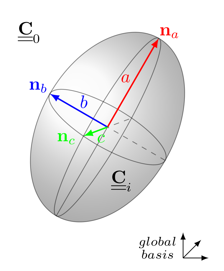
const auto P0_ellipsoid = computeHillPolarisationTensor<stress>(E0,nu0,n_a,a,n_b,b,c);Here, the first line computes the Hill tensor for a sphere. The
second one computes the Hill tensor for an axisymmetrical ellipsoid (or
spheroidal inclusion). The user must provide the normal vector
n_a for the axis, and e for the aspect ratio.
The third line computes the Hill tensor of a more general ellipsoid
whose semi-axis lengths are
a,b,c. The axis a is
related to direction given by n_a and b is
related to the direction given by n_b, which must be normal
to n_a (see the figure above).
An IsotropicModuli can also be passed for the
elasticity, as follows:
const auto IM0=YoungNuModuli<stress>(E0,nu0);
const auto P0 = computeSphereHillPolarisationTensor<stress>(IM0);
const auto P0_axi = computeAxisymmetricalHillPolarisationTensor<stress>(IM0,n_a,e);
const auto P0_ellipsoid = computeHillPolarisationTensor<stress>(IM0,n_a,a,n_b,b,c);
The Eshelby tensors can be computed as follows:
const auto S0 = computeSphereEshelbyTensor<stress>(nu0);
const auto S0_axi = computeAxisymmetricalEshelbyTensor<stress>(nu0,e);
const auto S0_ellipsoid = computeEshelbyTensor<stress>(nu0,a,b,c);
Note that the Eshelby tensors are not related to a basis, so that it is recommended to use the Hill tensors instead. In 2 dimensional framework, Eshelby tensors and Hill tensors are computed as follows:
const auto S0_D = computeDiskPlaneStrainEshelbyTensor<stress>(nu0);
const auto S0_C = computePlaneStrainEshelbyTensor<stress>(nu0,e);

const auto IM0=YoungNuModuli<stress>(E0,nu0);
const auto P0_D = computeDiskPlaneStrainHillTensor<stress>(IM0);
const auto P0_C = computePlaneStrainHillTensor<stress>(IM0,n_a,a,b);
The computeDiskPlaneStrain refers to a disk in plane
strain framework, whereas the computePlaneStrain refers to
an ellipse oriented by n_a, in a plane strain
framework.
The header LocalisationTensor.hxx also introduces the
computation of the strain localisation tensors of an ellipsoid. These
localisation tensors can be computed as follows:
const auto A = computeSphereLocalisationTensor<stress>(E0,nu0,Ei,nui);
const auto A_axi = computeAxisymmetricalLocalisationTensor<stress>(E0,nu0,Ei,nui,n_a,e);
const auto A_ellipsoid = computeLocalisationTensor<stress>(E0,nu0,Ei,nui,n_a,a,n_b,b,c);
Here, the subscript i refers to the inclusion. Here
again, an IsotropicModuli can be passed for the elasticity,
as follows:
const auto IM0=YoungNuModuli<stress>(E0,nu0);
const auto IMi=YoungNuModuli<stress>(Ei,nui);
const auto A = computeSphereLocalisationTensor<stress>(IM0,IMi);
const auto A_axi = computeAxisymmetricalLocalisationTensor<stress>(IM0,IMi,n_a,e);
const auto A_ellipsoid = computeLocalisationTensor<stress>(IM0,IMi,n_a,a,n_b,b,c);
Note that if the elasticity of the inclusion is not isotropic, an
anisotropic elasticity C_i can be provided, assuming that
this elasticity is expressed in the same basis as the one defined by
n_a,n_b (the local basis of the inclusion):
const auto A_aniso = computeLocalisationTensor<stress>(IM0,C_i,n_a,a,n_b,b,c);In 2 dimensional framework, localisation tensors are computed as follows:
const auto A_D = computeDiskPlaneStrainLocalisationTensor<stress>(IM0,C_i);
const auto A_C = computePlaneStrainLocalisationTensor<stress>(IM0,C_i,n_a,a,b);The header AnisotropicEshelbyTensor.hxx introduces the
computation of the Eshelby tensors and Hill tensors of general
ellipsoids embedded in an anisotropic medium. The anisotropic elasticity
\(\underline{\underline{\mathbf{C}}}_0\) must
be expressed in the global basis.
These tensors can be computed as follows:
const auto P0 = computeAnisotropicHillTensor<stress>(C0,n_a,a,n_b,b,c);
const auto P0_2d = computePlaneStrainAnisotropicHillTensor<stress>(C0,n_a,a,b);

const auto S0 = computeAnisotropicEshelbyTensor<stress>(C0,n_a,a,n_b,b,c);
const auto S0_2d = computePlaneStrainAnisotropicEshelbyTensor<stress>(C0,n_a,a,b);
The tensors are computed via an integration on a bi-dimensional
domain. The integration is iterative, and the user can provide the
number of iterations (basically, it corresponds to the number of
subdivisions in each domain direction). Hence, more iterations lead to
more accurate results, but take longer to compute. The default number of
iterations is 12, but it is recommended to increase it for
sharp ellipsoids:
const std::size_t it = 10;
const auto P0 = computeAnisotropicHillTensor<stress>(C0,n_a,a,n_b,b,c,10);
The localisation tensors are introduced in the same header
AnisotropicEshelbyTensor.hxx. We can do as follows:
const auto A = computeAnisotropicLocalisationTensor<stress>(C0_glob,Ci_loc,n_a,a,n_b,b,c);
const auto A_2d = computePlaneStrainAnisotropicLocalisationTensor<stress>(C0_glob,Ci_loc,n_a,a,b);
The user must provide the elasticity of the inclusion as a
st2tost2 Ci_loc, and if it is not isotropic,
it must be provided in the local basis defined by
n_a,n_b.
Note that the functionalities below are also available in the
Python module (see the doc here).
See also here a tutorial
on the computation of homogenized schemes for biphasic particulate
microstructures.
Different classical mean-field homogenization schemes are implemented
for biphasic media. These schemes are introduced by the header
LinearHomogenizationSchemes.hxx. They only deal with
isotropic matrices and locally isotropic inclusions (for anisotropic
matrices or inclusions, see the section “Homogenization of general
microstructures”).
The available schemes are:
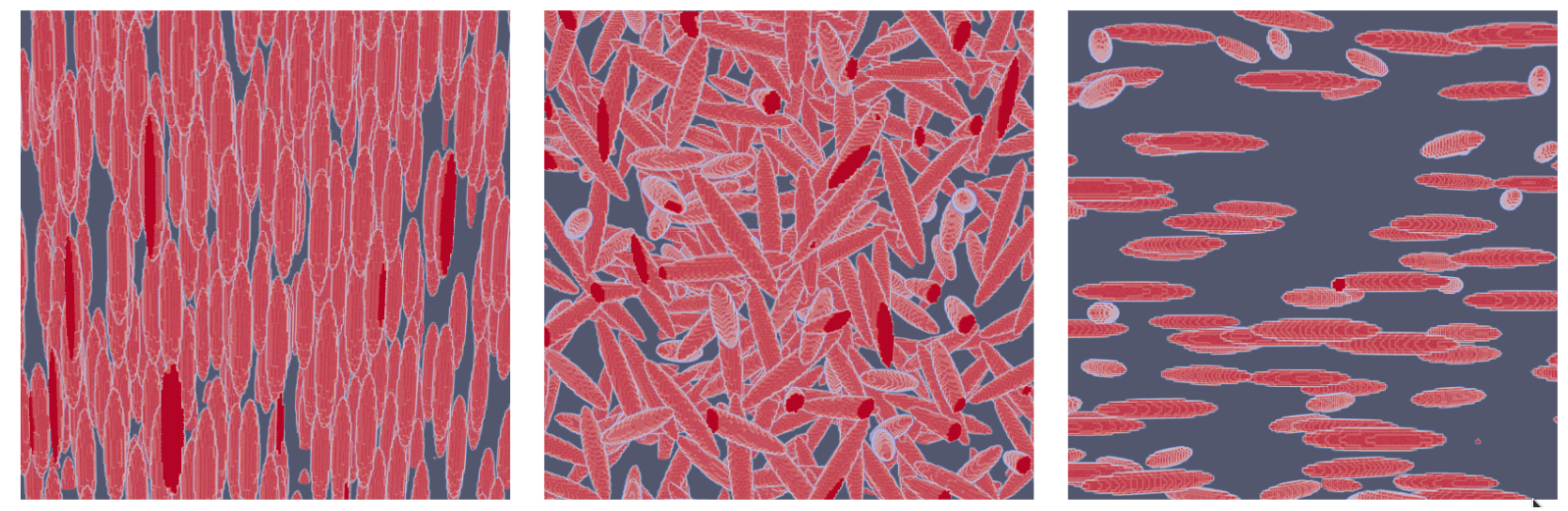
Each scheme is based on the average of the localisation tensor \(\underline{\underline{\mathbf{A}}}_i\) defined above. This average is computed assuming different distributions of ellipsoids. Hence, different cases are considered:
Hence we can compute the homogenized stiffness returned by the available schemes. For example, for the distribution of spheres:
const auto IM0=YoungNuModuli<stress>(E0,nu0);
const auto IMi=YoungNuModuli<stress>(Ei,nui);
const auto KG_DS = computeSphereDiluteScheme<stress>(IM0,f,IMi);
const auto KG_MT = computeSphereMoriTanakaScheme<stress>(IM0,f,IMi);
Note that the two above schemes return a KGModuli object
(see above).
Also, f is the volume fraction, and the subscript
0 refers to the matrix, and the subscript i
refers to the inclusion.
For the oriented inclusions, we can do:
const auto C_DS = computeOrientedDiluteScheme<stress>(IM0,f,IMi,n_a,a,n_b,b,c);
const auto C_MT = computeOrientedMoriTanakaScheme<stress>(IM0,f,IMi,n_a,a,n_b,b,c);
const auto C_PCW = computeOrientedPCWScheme<stress>(IM0,f,IMi,n_a,a,n_b,b,c,D);
Here, the three above schemes return st2tost2 objects.
Note that PCW refers to the Ponte-Castaneda and Willis
scheme. For this scheme, a Distribution object must be
created by the user. It is defined by two vectors \(\underline{n}_a,\underline{n}_b\) and three
lengths \(a,b,c\) that define the
ellipsoid which defines the distribution:
Distribution<stress> D = {.n_a = n_a, .a = a, .n_b = n_b, .b = b, .c = c};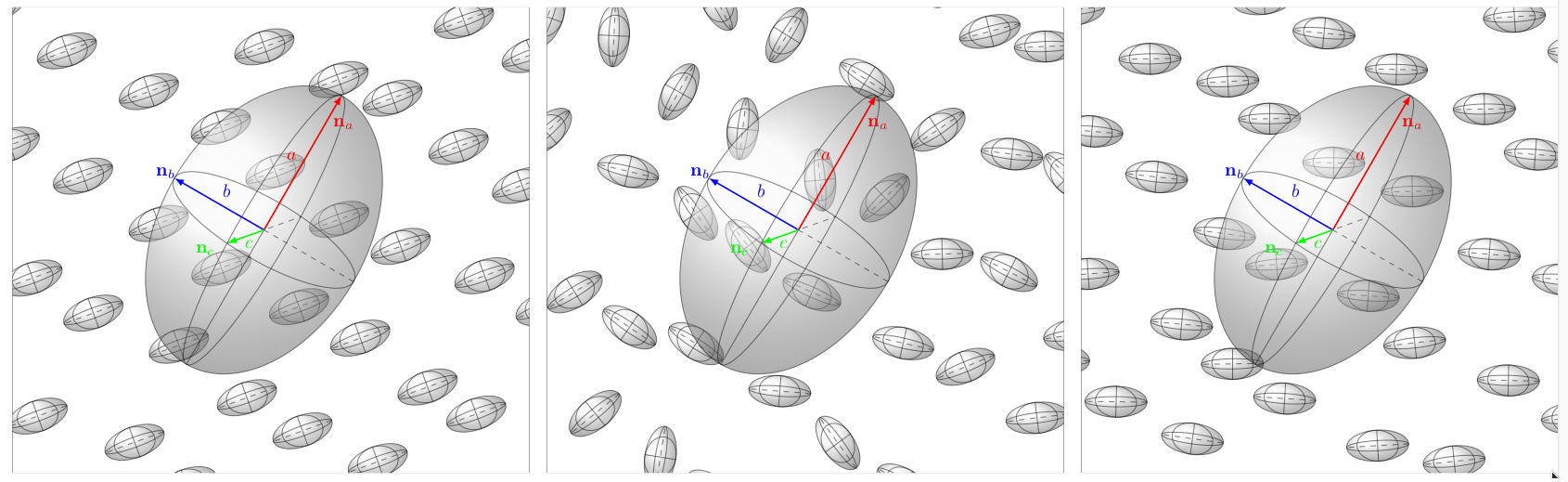
Indeed, in the Ponte-Castaneda and Willis scheme, there is a
difference between the ellipsoid which defines the distribution of the
inclusions, and the ellipsoid which defines the shape of the inclusions
(in the image above, we represent the distribution D of
inclusions by a big ellipsoid, with colored axes). A bigger axis for
D means that along this axis, the distribution of
inclusions is more diluted. A short axis means that, on the contrary,
the distribution is denser along this axis.
For the isotropic distribution of ellipsoids, we can do:
const auto KG_DS = computeIsotropicDiluteScheme<stress>(IM0,f,IMi,a,b,c);
const auto KG_MT = computeIsotropicMoriTanakaScheme<stress>(IM0,f,IMi,a,b,c);
const auto C_PCW = computeIsotropicPCWScheme<stress>(IM0,f,IMi,a,b,c,D);
Here, the two first schemes return KGModuli objects,
whereas computeIsotropicPCWScheme returns a
st2tost2 object. For this latter case, the ellipsoids have
indeed a uniform isotropic distribution of orientations, but the user
might use a non-isotropic Distribution D (it corresponds to
the configuration at the center on the image). And finally, we can
consider a transverse isotropic distribution of inclusions:
const auto C_DS = computeTransverseIsotropicDiluteScheme<stress>(IM0,f,IMi,n_a,a,b,c);
const auto C_MT = computeTransverseIsotropicMoriTanakaScheme<stress>(IM0,f,IMi,n_a,a,b,c);
const auto C_PCW = computeTransverseIsotropicPCWScheme<stress>(IM0,f,IMi,n_a,a,b,c,D);
Here, the three above schemes return st2tost2 objects.
Because the functions are based on the average of the localisation
tensor \(\underline{\underline{\mathbf{A}}}_i\)
associated with each distribution, a Base function is also
defined for each scheme, that only takes in argument the average of the
localisation tensor A_av. We then can compute a homogenized
stiffness with a very general averaged localisator:
const auto C_DS = computeDiluteScheme<stress>(E0,nu0,f,Ei,nui,A_av);
const auto C_MT = computeMoriTanakaScheme<stress>(E0,nu0,f,Ei,nui,A_av);
const auto C_PCW = computePCWScheme<stress>(E0,nu0,f,Ei,nui,A_av,D);
Here, the three above schemes return st2tost2
objects.
Different bounds are implemented and are introduced by the header
LinearHomogenizationBounds.hxx. The available bounds
are:
Here are some examples of computation:
//Voigt and Reuss bounds
std::vector<real> tab_f={real(0.2),real(0.8)};
const auto C0 = stress(1e9)*Stensor4<3u,real>::Id();
const auto C1 = stress(1e7)*Stensor4<3u,real>::Id();
std::vector<Stensor4<3u,stress>> tab_C={C0,C1};

const Stensor4<3u,real> CV = computeVoigtStiffness<3u, stress>(tab_f, tab_C);
const Stensor4<3u,real> CR = computeReussStiffness<3u, stress>(tab_f, tab_C);

//Hashin-Shtrikman bounds
const auto K0=stress(1/3);
const auto G0=stress(1/2);
const auto K1=stress(2/3);
const auto G1=stress(1);
const auto K2=stress(5/3);
const auto G2=stress(5/2);
std::vector<real> tab_f={real(0.1),real(0.8),real(0.1)};
std::vector<stress> tab_K={K0,K1,K2};
std::vector<stress> tab_mu={G0,G1,G2};

const auto pair = computeIsotropicHashinShtrikmanBounds<3u, stress>(tab_f, tab_K, tab_mu);

const auto LB = std::get<0>(pair);
const auto K_L = std::get<0>(LB);
const auto mu_L = std::get<1>(LB);

const auto UB = std::get<1>(pair);
const auto K_U = std::get<0>(UB);
const auto mu_U = std::get<1>(UB);
Note that Voigt and Reuss bounds work on st2tost2 (or
Stensor4) objects, whereas Hashin-Shtrikman bounds work on
bulk and shear moduli. The number of phases is arbitrary, and the
dimension is 2 or 3.
Some functions (defined in the header HomogenizationSecondMoments.hxx) allow to compute the second moments of the strains when considering a Hashin-Shtrikman type microstructure. More precisely, we consider isotropic spherical inclusions embedded in an isotropic matrix, and we compute the following moments:
\(\langle\varepsilon_{eq}^2\rangle_r\qquad\text{and}\qquad\langle\varepsilon_{m}^2\rangle_r\)
on each phase \(r\), \(\varepsilon_{eq}\) being the equivalent strain and \(\varepsilon_{m}\) being the third of the trace of the strain. We hence write
const auto kg0 = KGModuli<stress>(K0,G0);
const auto kgr = KGModuli<stress>(K1,G1);
using namespace tfel::material::homogenization::elasticity;
const auto em2r = computeMeanSquaredHydrostaticStrain(kg0,fr,kgr,em2,eeq2);
const auto em20=std::get<0>(em2);
const auto em2i=std::get<1>(em2);
const auto eeq2r = computeMeanSquaredEquivalentStrain(kg0,fr,kgr,em2,eeq2);
const auto eeq20=std::get<0>(eeq2);
const auto eeq2i=std::get<1>(eeq2);
Here the functions appearing at lines 4 and 7 need 5 arguments:
isotropic modulus of the matrix kg0, volume fraction of
spheres, isotropic modulus of the inclusions kgr, but also
the second moments of the total strain: em2 for the
hydrostatic part and eeq2 for the deviatoric part. The
functions return std::pair, each element of the
pair corresponds to a phase (matrix or spheres).
A ParticulateMicrostructure object can be created for
homogenization of general matrix-inclusion microstructures. Note that
the functionalities below are also available in the Python
module (see the doc here).
ParticulateMicrostructure classThe ParticulateMicrostructure class is available in 3d
an 2d via 2 template parameters:
ParticulateMicrostructure<N,stress> with
N the dimension. For the details, see the file
‘MicrostructureDescription.hxx’ which introduces the
class.
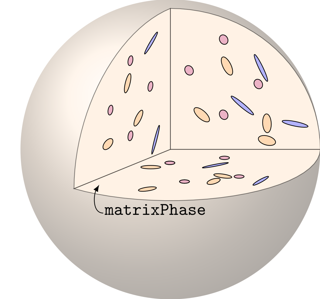
A ParticulateMicrostructure consists of a matrix, in
which are embedded several distributions of inclusions. The class has
three (private) attributes:
number_of_phasesmatrix_phaseinclusion_phasesThe matrix_phase is of type Phase,
described below.
The inclusion_phases is a std::vector of
pointers on InclusionDistribution objects (which represent
the distributions of inclusions). This class is also described
below.
We can instantiate a ParticulateMicrostructure as
follows, passing the matrix elasticity as an argument:
using namespace tfel::material::homogenization::elasticity;
const auto IM0=tfel::material::KGModuli<stress>(1e7,1e7);
const auto micro_1=ParticulateMicrostructure(IM0);

const auto C0 = stress(1e9)*Stensor4<3u,real>::Id();
const auto micro_2=ParticulateMicrostructure(C0);
ParticulateMicrostructure has also some methods (see
‘MicrostructureDescription.hxx’ for details). The following ones allow
to get some attributes of the class:
getNumberOfPhasesgetMatrixFraction (attribute fraction of
matrix_phase)getMatrixElasticity (attribute stiffness
of matrix_phase)isIsotropicMatrix (private attribute
isotropic of matrix_phase)The last method returns a boolean which states if the matrix is
considered isotropic or not. In fact, depending on how the
ParticulateMicrostructure was instantiated, the matrix is
considered isotropic or not. For example, by doing
bool val_1=micro_1.isIsotropicMatrix();
bool val_2=micro_2.isIsotropicMatrix();
val_1 will be True because
micro_1 was instantiated above with a
KGModuli, whereas val_2 will be
False. Note that False does not mean that the
matrix elasticity is not isotropic, but that it is CONSIDERED as not
isotropic.
Other methods allow to add/remove InclusionDistribution
objects to the attribute inclusion_phases, and also to
modify the properties of the phases:
getInclusionPhaseaddInclusionPhaseremoveInclusionPhasechangeElasticityOfMatrixPhasechangeElasticityOfInclusionPhasechangeFractionOfInclusionPhaseBut we first describe Phase,
InclusionDistribution and Inclusion
classes.
Phase classThe Phase class has three attributes:
fraction (real type)isotropic (bool type, private
attribute)stiffness (st2tost2 type, private
attribute)and three methods:
isIsotropicchangeElasticityOfPhasegetElasticityOfPhaseisIsotropic() returns a bool stating if the
phase is considered isotropic or not. Again, the value of this
bool depends on the way the Phase was
constructed. By doing
const auto C0=tfel::math::st2tost2<stress>::Id();
Phase<stress> ph(f,C0);
bool b = ph.isIsotropic();
b will have the value false, whereas by
doing
const auto KG=tfel::material::KGModuli<stress>(k,g);
Phase<stress> ph(f,KG);
bool b = ph.isIsotropic();
b will have the value true. Hence, when a
ParticulateMicrostructure is instantiated, it automatically
instantiates a Phase object corresponding to the attribute
matrix_phase. However, we note that the user can construct
a microstructure without using Phase instantiation
directly.
Inclusion classBefore describing the InclusionDistribution class, we
must describe the Inclusion class. This latter is
characterized by its unique attribute: semiLengths. It is a
std::array of N lengths, which are the
semi-lengths of the ellipsoid/ellipse, where N is the
dimension considered (2 or 3). Hence, Inclusion has two
template parameters: Inclusion<N,LengthType>. Some
particular Inclusion objects are also defined:
Ellipsoid (child of Inclusion in 3d)Spheroid (child of Ellipsoid with the last
two semi-lengths identical)Sphere (child of Spheroid with 3
semi-lengths equal to unity)Let us try:
Ellipsoid<length> ellipsoid1(a,b,c);
Spheroid<length> spheroid1(a,b);
Sphere<length> sphere1();InclusionDistribution classThe InclusionDistribution class is an abstract class
which represents a distribution of inclusions. It is a child of the
Phase class, and it is used to represent the distribution
of inclusions in a ParticulateMicrostructure. There are 4
child class of the
InclusionDistribution class:
SphereDistribution (distribution of spheres)IsotropicDistribution (isotropic distribution of
ellipsoids)TransverseDistribution (transverse isotropic
distribution of ellipsoids)OrientedDistribution (aligned distribution of
ellipsoids)UserDefinedDistributionOfSpheroids (distribution of
spheroids defined with orientation tensors)Here are some examples of instantiation:
const auto KGi=tfel::material::KGModuli<stress>(Ki,Gi);
SphereDistribution<stress> distrib_sph(sphere1,f,KGi);
IsotropicDistribution<stress> distrib_ell(ellipsoid1,f,KGi);

tfel::math::tvector<3u, real> n_a = {1., 0., 0.};
tfel::math::tvector<3u, real> n_b = {0., 1., 0.};
OrientedDistribution<stress> distrib_O(ellipsoid1,f,KGi,n_a,n_b);
The TransverseDistribution is a special case which
requires specifying which axis of the ellipsoid (or spheroid) will
remain fixed when the two other axes rotate:
unsigned short int index = 0;
TransverseIsotropicDistribution<stress> distrib_TI(ellipsoid1,f,KGi,n_a,index);
The index can be 0,1 or 2. For a spheroid, giving 2 for
the index is the same as giving 1, because
these 2 axes have the same length.
Note that the OrientedDistribution can be instantiated
with a Stensor4 object as elasticity. It is also possible
for a SphereDistribution. It can be useful for considering
anisotropic inclusions. However, the basis in which the
Stensor4 elasticity is defined is the local basis for the
OrientedDistribution, that is, the basis defined by
n_a and n_b passed as arguments. For a
SphereDistribution, it is the global basis.
The UserDefinedDistributionOfSpheroids is a distribution
of Spheroid (3d-objects, with two equal axes, see above).
It is defined with two tensors: a second-order tensor \(\underline{A}_2\) and a fourth-order tensor
\(\underline{A}_4\):
\[ \underline{A}_2=\langle\vec n\otimes\vec n\rangle\qquad\underline{A}_4=\langle\vec n\otimes\vec n\otimes\vec n\otimes\vec n\rangle \]
This distribution can be instantiated as follows, with the help of the Walpole Basis (see here the documentation).
using namespace tfel::math;
tvector<3u, real> n_a = {1., 0., 0.};
tvector<3u, real> n_b = {0., 1., 0.};
const stensor<3u,real> A2 = 1./2*TransverseIsotropicWalpoleBasis<real>::q(n_b);

const auto E2d=TransverseIsotropicWalpoleBasis<real>::E2(n_b);
const auto Fd=TransverseIsotropicWalpoleBasis<real>::F(n_b);
const st2tost2<3u,real> A4 = 1./2*E2d+1./4*Fd;

UserDefinedDistributionOfSpheroids<stress> distribution(spheroid1, f, KGi, A2, A4);
We can now construct our ParticulateMicrostructure by
adding some InclusionDistribution objects:
micro_1.addInclusionPhase(distrib_sph);
std::cout<< micro_1.getNumberOfPhases()<< std::endl;
std::cout<< micro_1.getMatrixFraction()<< std::endl;

micro_1.addInclusionPhase(distrib_ell);
std::cout<< micro_1.getNumberOfPhases()<< std::endl;
std::cout<< micro_1.getMatrixFraction()<< std::endl;
or remove them:
micro_1.removeInclusionPhase(0);
std::cout<< micro_1.getNumberOfPhases()<< std::endl;
std::cout<< micro_1.getMatrixFraction()<< std::endl;
At this stage, we have added the distribution of spheres
distrib_sph, and added the isotropic distribution of
ellipsoids distrib_ell. After that, we have removed the
first inclusion distribution (number 0), which is the
distribution of spheres. Hence, only one
InclusionDistribution object remains in the microstructure.
We can get this distribution by doing:
const auto ell_dist=micro_1.getInclusionPhase(0);Each InclusionDistribution object has three attributes:
inclusion (which is of type Inclusion, see
above), fraction and stiffness (because they
are attributes of Phase objects). It has also two methods.
The first just states if the distribution was instantiated with an
IsotropicModuli or with a Stensor4 object.
Here, it was instantiated with a KGModuli, so that it is
considered isotropic. Hence,
std::cout<< ell_dist.isIsotropic()<< std::endl;prints 1.
The second method of the distribution allows to compute the mean strain localisation (or concentration) tensor in the inclusions when they are embedded in a matrix:
Ai=ell_dist.computeMeanLocalisator(IM0);Note that in the latter case, passing C0, a
Stensor4 object as an argument of the method will return an
error, because it will be considered that the matrix is not isotropic,
so that computing an average localisator of a distribution of ellipsoids
in an anisotropic matrix is impossible (too complicated). However, it
can be done for other kinds of distributions, like sphere distributions
or distributions of oriented inclusions:
A1=distrib_sph.computeMeanLocalisator(C0,10);
A2=distrib_O.computeMeanLocalisator(C0,10);
Here, the integer 10 is the number of subdivisions in
the integration process in the computation of the Hill tensor relative
to the inclusions. It is 12 by default.
A last method of the ParticulateMicrostructure object
allows to change the elasticity of the matrix phase:
micro_1.changeElasticityOfMatrixPhase(C0);
std::cout<< micro_1.getMatrixElasticity()<< std::endl;
std::cout<< micro_1.isIsotropicMatrix()<< std::endl;
Here we see that the matrix is no more isotropic because it was
replaced via a Stensor4 object C0.
Note that the 4 InclusionDistribution classes are
currently available in 3d only.
The file MicrostructureLinearHomogenization.ixx
introduces a HomogenizationScheme object which has three
attributes:
homogenized_stiffnesseffective_polarisationmean_strain_localisation_tensorsThis is the object that the functions listed below return:
computeDilute (dilute scheme)computeMoriTanaka (Mori-Tanaka scheme)computeSelfConsistent (Self-Consistent scheme)These functions take a ParticulateMicrostructure as an
argument and returns a HomogenizationScheme object.
Let us try:
using namespace tfel::material::homogenization::elasticity;
auto hmDS=computeDilute<3u,stress>(micro_1);
auto hmMT=computeMoriTanaka<3u,stress>(micro_1);
auto hmSC=computeSelfConsistent<3u,stress>(micro_1,1e-6,true);
We note that computeSelfConsistent not only takes the
microstructure as an argument, but also takes one real
(1e-6) as a parameter, which pilots the accuracy of the
result. Indeed, at each iteration of the self-consistent iterative
algorithm, the function computes the relative difference between the new
and the old homogenized stiffness. This relative difference must be
smaller than the tolerance given as a parameter. Moreover, the
bool parameter (true) precises if the
computation considers an isotropic matrix when computing the Hill
tensors relative to the inclusions, at each iteration of the algorithm.
Indeed, the homogenized stiffness may be non isotropic, so that the user
can make the choice of isotropizing this homogenized stiffness at each
iteration. Otherwise, he can put false, so that a numerical
integration (resulting in a slower computation) will be performed to
compute the Hill tensors. Moreover, an integer parameter can be added
after the boolean, that indicates the number of subdivisions in the
numerical integration. This value is 12 by default:
micro_2.addInclusionPhase(distrib_O);
hmSC_iso=computeSelfConsistent<3u,stress>(micro_2,10,true);
hmSC_aniso=computeSelfConsistent<3u,stress>(micro_2,10,false,10);
std::cout<< "SC iso: "<< hmSC_iso.homogenized_stiffness<< std::endl;
std::cout<< "SC aniso: "<< hmSC_aniso.homogenized_stiffness<< std::endl;
(the “std::cout” does not work when using quantities). For the other
schemes, the isotropic character of the matrix when computing the strain
localisators will depend on what
micro_1.isIsotropicMatrix() returns. Hence, it is important
to initialize the matrix or the microstructure with the appropriate
elastic moduli. If isotropic, it will work in all cases, whereas if not
isotropic, it will fail depending on the distributions that are present
in the microstructure. Moreover, if anisotropic, another parameter can
be passed to specify the number of subdivisions in the numerical
integration (this value is 12 by default):
micro_1.changeElasticityOfMatrixPhase(C0);
micro_1.removeInclusionPhase(0);
micro_1.addInclusionPhase(distrib_O);
auto hmDS_aniso=computeDilute<3u,stress>(micro_1,10);
auto hmMT_aniso=computeMoriTanaka<3u,stress>(micro_1,10);
We can recover the strain localisation tensors as follows:
A_i_DS=hmDS.mean_strain_localisation_tensors;
std::cout<<"A_0_DS: "<< A_i_DS[0]<<"A_1_DS: "<< A_i_DS[1]<< std::endl;
We can also add a polarization on each phase:
micro_1.changeElasticityOfMatrixPhase(IM0);
const auto P0 = Stensor<3u,stress>::zero();
const Stensor<3u,stress> P1 = {stress(6.e8),stress(6.e8),stress(6.e8),stress(0.),stress(0.),stress(0.)};
const auto pola={P0,P1};
auto hmDS_pola=computeDilute<3u,stress>(micro_1,0,pola);
Note that here we must also specify the parameter
max_iter_anisotropic_integration before the optional
argument pola. Here this integer is 0 because it will not
be used, given that the matrix phase is isotropic (see first line). And
we can recover the effective polarization:
auto P_eff_DS=hmDS_pola.effective_polarisation;