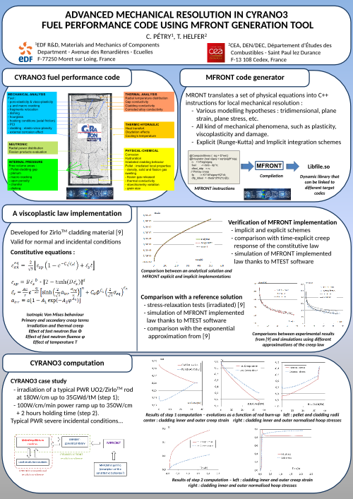
Cyrano3 interfaceThe industrial reference software CYRANO3 has been developed by EDF for more than 20 years to simulate the PWR fuel thermo-mechanical behaviour under nominal and incidental conventional operating conditions (See [1]).
The code integrates extensive knowledge and know-how based on more than 30 years of national and international research and feedback in the framework of nuclear materials under irradiation. It is part of the PLEIADES platform jointly developed by EDF and CEA, and validated on an extensive database including more than 900 irradiated fuel rods examination and validation results.
The cyrano interface for material properties generates
function having the following prototype:
~~{.c++} CyranoRealType ()(CyranoOutputStatus const,
const CyranoRealType* const, const CyranoIntegerType, const
CyranoOutOfBoundsPolicy);~~
The first argument contains the output status (see Section 1.1 for details).
The second argument contains the arguments of the material property.
The third argument gives the number of arguments.
The fourth argument specify the policy used when an argument or the output is out of these bounds.
On error, the returned value is Not A Number
(Nan).
Full diagnostic is available in the CyranoOutputStatus
structure. See the doxygen
documentation.
The CyranoOutOfBoundsPolicy is an enumeration of the
available policies. Three policies are declared:
CYRANO_NONE_POLICY: with this policy, nothing is done
if the arguments are out of their bounds (checks are not even
performed).CYRANO_WARNING_POLICY: with this policy, checks on the
arguments are performed. If one argument is out of its bounds, this will
be reported in the output status and an appropriate error message will
be reported. The computations are however performed.CYRANO_STRICT_POLICY: With this policy, checks on the
arguments are performed. If one argument is out of its bounds, this will
be reported in the output status and an appropriate error message will
be reported.
The interface with MFront has been presented during the LWR Fuel Performance Meeting in 2015 (Zurich, Switzerland), see [2]:
The Cyrano3 code is based on a 1D description of the
fuel rods using a finite element kernel to solve the thermal and
mechanical radial equilibrium at different axial positions.

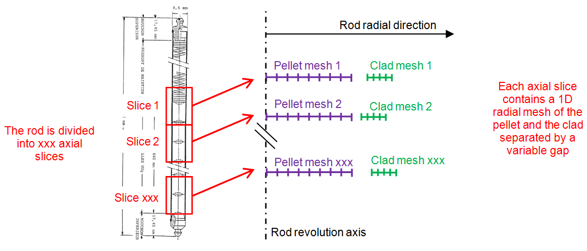
The principle of the geometrical discretisation of a single rod is illustrated in Figure 1. Due to revolution axisymmetry, only radial and axial directions are discretised. The fuel rod is axially divided in slices, leading to the so-called “1,5D” typical axisymmetric scheme - each slice being represented by a one-dimensional radial mesh including a pellet and a clad separated by a variable gap.
To solve the mechanical equilibrium of a slice, two distinct hypotheses concerning the axial direction are supported:
Cyrano3 finite strain modelling is based on the approach
described by T. Helfer (See [3]) which allows to easily
extend small strain mono-dimensional code to support finite strain
modelling.
This approach relies on the fact that the direct link between the deformation gradient \({\underset{\tilde{}}{\mathbf{F}}}\) and the linearized strain \(\underline{\varepsilon}^{\mathrm{to}}\) in monodimensional modelling:
\[ {\underset{\tilde{}}{\mathbf{F}}} = {\underset{\tilde{}}{\mathbf{I}}} + \underline{\varepsilon}^{\mathrm{to}} \]
The mechanical equilibrium is expressed in the reference configuration:
\[ \mathop{\mathrm{Div}}{\underset{\tilde{}}{\mathbf{\Pi}}} = \vec{0} \]
where :
If \({{\mathrm{d}}}\,\vec{f}\) is the force applied to an infinitesimal surface \({{\mathrm{d}}}\,\vec{s}\) in the current configuration which maps to the infinitesimal surface \({{\mathrm{d}}}\,\vec{S}_{0}\) in the reference configuration, the first Piola-Kirchoff stress \({\underset{\tilde{}}{\mathbf{\Pi}}}\) has the following property:
\[ {{\mathrm{d}}}\,\vec{f}={\underset{\tilde{}}{\mathbf{\Pi}}}\,\colon\,{{\mathrm{d}}}\,\vec{S}_{0} \]
For pressure loading, one have: \[ {{\mathrm{d}}}\,\vec{f}=-P\,{{\mathrm{d}}}\,\vec{s} \]
In 1D, the normal is constant, so the radial component \(\Pi_{rr}\) of \({\underset{\tilde{}}{\mathbf{\Pi}}}\) satisfies:
\[ \Pi_{rr}=-P\,{{\displaystyle \frac{\displaystyle S}{\displaystyle S_{0}}}} \]
Here, the surface is defined by: \[ S=2\,\pi\,R\,H \] where \(R\) is the actual radius and \(H\) is the actual height. Thus,
\[ \Pi_{rr}=-P\,{{\displaystyle \frac{\displaystyle R}{\displaystyle R_{0}}}}\,{{\displaystyle \frac{\displaystyle H}{\displaystyle H_{0}}}}=-P\,\left(1+{{\displaystyle \frac{\displaystyle u_r\left(R_{0}\right)}{\displaystyle R_{0}}}}\right)\,\varepsilon^{\mathrm{to}}_{zz} \]
where \(u_{r}\) is the radial displacement, \(R_{0}\) is the initial radius and \(\varepsilon^{\mathrm{to}}_{zz}\) is the axial strain.
These relations are exactly the same as in small strain analysis, except for the dependency of \(S\) with the actual radius which adds additional terms to the stiffness matrix.
In generalised plane stress, the axial strain is not known. As discussed later, the axial strain is generally computed by the behaviour to ensure that the axial stress is equal to the prescribed value. This provides a way to compute the axial strain for the computation of the radial force, but one can not derive the exact stiffness matrix of the system. Another simpler solution is to consider the axial strain as constant during the time step for the computation of the radial forces.
For a closed pipe, the axial force applied to the tube can be computed as follows:
\[ F = P_{i}\,S^{c}_{i} - P_{e}\,S^{c}_{e} \]
where:
Here, the pressure is assumed constant over the time step : the
sensibility with the geometrical changes is neglected. Dependency of the
pressure with the volume can also be taken into account, as in
MTest if all the slices are homogeneous, which is almost
never the case.
In generalised plane stress, \(\Pi_{zz}\) is assumed uniform and can determined by:
\[ F = \Pi_{zz}\,\left(\left(S^{c}_{e}\right)^{0}-\left(S^{c}_{i}\right)^{0}\right) = P_{i}\,S^{c}_{i} - P_{e}\,S^{c}_{e} \]
This relation is exactly the same as in small strain analysis, except for the dependency of \(S^{c}_{i}\) and \(S^{c}_{e}\) with the actual inner and outer radius which adds additional terms to the stiffness matrix.
In generalised plane strain, the total force is given by:
\[ F = 2\,\pi\,\int_{R_{i}^{0}}^{R_{e}^{0}}\Pi_{zz}\,R\,dR = P_{i}\,S^{c}_{i} - P_{e}\,S^{c}_{e} \]
This is exactly the same relation as in same strain analysis, except for the dependency of \(S^{c}_{i}\) and \(S^{c}_{e}\) with the actual inner and outer radius which adds additional terms to the stiffness matrix
Currently, the MFront interface only supports
strain-based behaviour based on the Hencky strain measure, as described
by Miehe et al. (See [4]).
The Hencky strain measure is defined by:
\[ \underline{\varepsilon}_{\log}^{\mathrm{tot}}={{\displaystyle \frac{\displaystyle 1}{\displaystyle 2}}}\,\log{{{\underset{\tilde{}}{\mathbf{F}}}^{\mathop{T}}}\,\cdot\,{\underset{\tilde{}}{\mathbf{F}}}} \]
In \(1D\), this relation boils down to (See [3]):
\[ \left(\underline{\varepsilon}^{\mathrm{to}}_{\text{log}}\right)_{i}=\log\left(1+\underline{\varepsilon}^{\mathrm{to}}_{i}\right) \]
Based on energetic consideration, this strain measure also defined its dual stress denoted \(\underline{T}\). The relation between \({\underset{\tilde{}}{\mathbf{\Pi}}}\) and \(\underline{T}\) is fairly complex in \(3D\), but quite simple in \(1D\):
\[ \Pi_{i} = {{\displaystyle \frac{\displaystyle T_{i}}{\displaystyle 1+\left(\underline{\varepsilon}^{\mathrm{to}}\right)_{i}}}} \]
The generalised plane stress hypothesis is treated by introducing, at each integration point, an additional unknown: the axial logarithmic strain. Using the previous equations, the implicit equation associated with this unknown is:
\[ \exp\left( \left.\left(\underline{\varepsilon}^{\mathrm{to}}_{\text{log}}\right)_{zz}\right|_{t}+ \Delta\,\left(\underline{\varepsilon}^{\mathrm{to}}_{\text{log}}\right)_{zz} \right) \,\left.T_{zz}\right|_{t+\Delta\,t}= \left.\Pi_{zz}^{(i)}\right|_{t+\Delta\,t} \]
where \(\Pi_{zz}^{(i)}\) is the prescribed axial stress.
This equation is automatically added by the Hooke stress potential
used by the StandardElasticity and
StandardViscoplasticity bricks.
Elastic prediction of the stress
Most stress potentials provide a
computeElasticPredictionmethod. Under the generalised plane stress hypothesis and using the logarithmic strain, this method becomes non-linear. The total axial logarithmic strain is computed so that: \[ \exp\left( \left.\left(\underline{\varepsilon}^{\mathrm{to}}_{\text{log}}\right)_{zz}\right|_{t}+ \Delta\,\left(\underline{\varepsilon}^{\mathrm{to}}_{\text{log}}\right)_{zz}\right) \,\left.T_{zz}^{el}\right|_{t+\Delta\,t}= \left.\Pi_{zz}^{(i)}\right|_{t+\Delta\,t} \] where \(\left.T_{zz}^{el}\right|_{t+\Delta\,t}\) is the elastic prediction of the stress, computed as a function of \(\left(\Delta\,\underline{\varepsilon}^{\mathrm{to}}_{\text{log}}\right)_{zz}\) among other variables (elastic strain at the beginning of the time step, in plane total strain increment, etc…)The elastic prediction of the stress is then based on the following approximation of the elastic strain at the middle of the time step: \[ \left.\underline{\varepsilon}^{\mathrm{el}}\right|_{t}+\theta\, \left(\Delta\,\underline{\varepsilon}^{\mathrm{to}}-\Delta\underline{\varepsilon}^{sf}\right) \] where \(\Delta\underline{\varepsilon}^{sf}\) is the increment of all the stress strains (thermal expansion, swelling, and so on.)