MFront and MGIS in 2020TFEL, MFront and MTestTFEL libraries
MFront
MTest
python bindings
tfel-unicode-filttfel-configStandardElastoViscoPlasticity brickMTestgeneric
behavioursMFrontconst correctness in the generic
behaviour@GasEquationOfState keywordTFEL targets for use by external projectsStandardElastoviscoPlascity brickStandardElastoviscoPlascity brickNaNThe page describes the new functionalities of Version 3.4 of the
TFEL project.
MFront and MGIS in 2020
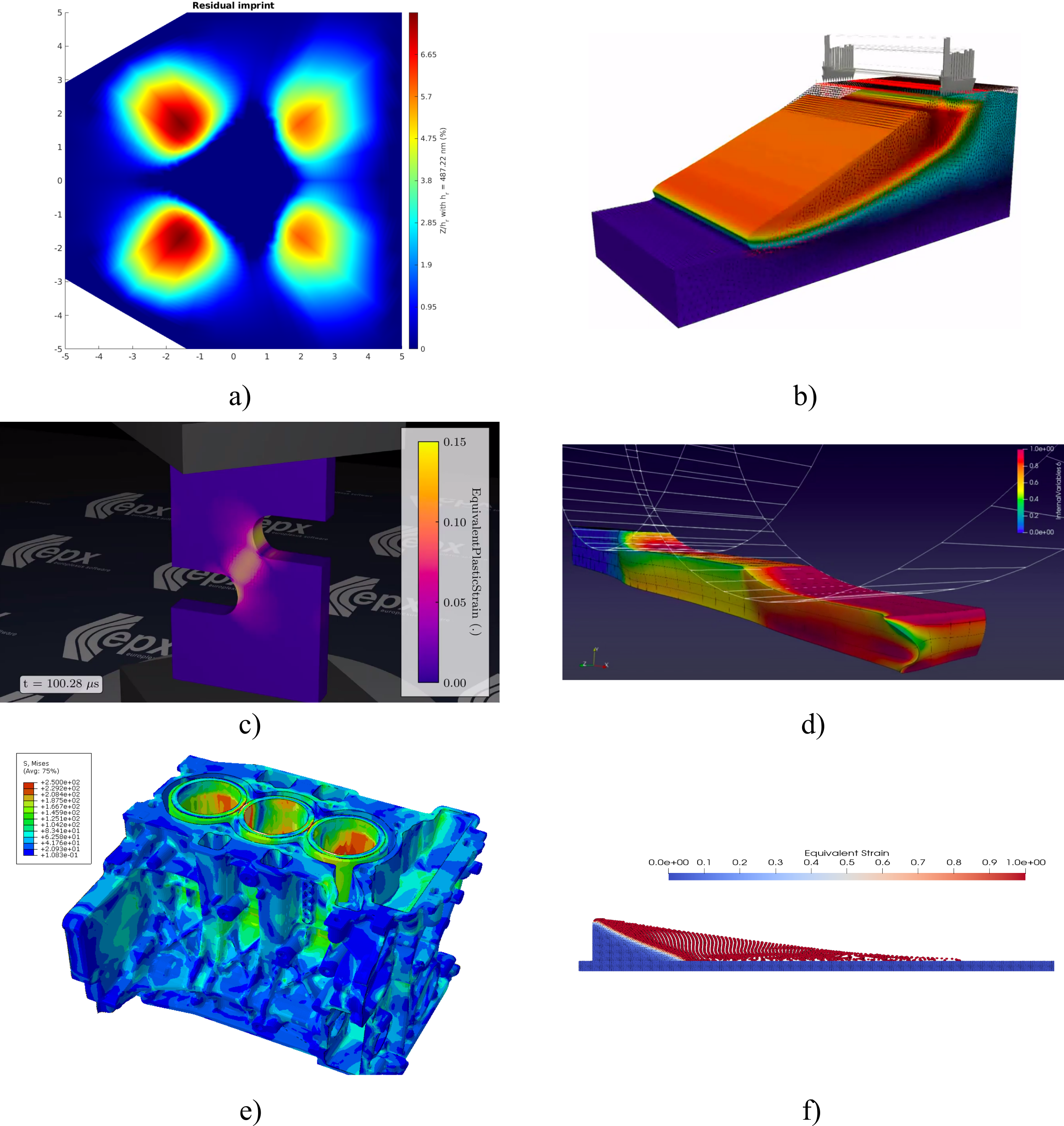
MFront and MGIS in 2020Figure 1 presents some noticeable applications of
MFront:
Ansys. Contribution of A. Bourceret and A. Lejeune,
(FEMTO).OpenGeoSys [2].
Contribution of T. Deng and T. Nagel (Geotechnical Institute, Technische
Universität Bergakademie Freiberg).MGIS integration in
Europlexus. Contribution of P. Bouda, (CEA DM2S).MEFISTO. Contribution of O. Jamond, (CEA DM2S).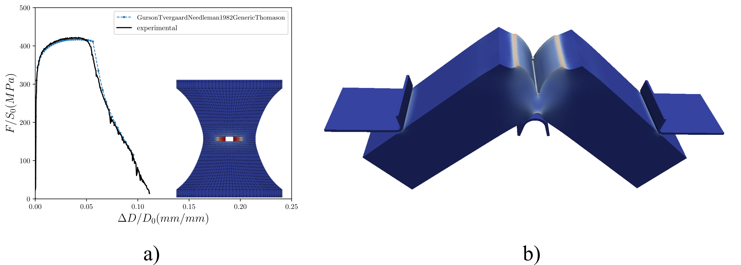
Cast3M simulation of a Notched
Tensile sample of an AA6061-T6 found in the core of Jules Horowitz
Reactor and comparison of simulation result with experimental data. b)
Cast3M simulation of a Charpy test on the PWR reactor core
vessel’ steelThe major features of Version 3.4 are:
StandardElastoViscoPlasticity
brick to porous materials See Figure 2 for some examples of ductile
failure simulations with Cast3M.MFront behaviours in a madnex file.
madnex is a data model based on HDF5 file
format that was originally designed by EDF as part of their in-house
projects for capitalising their experimental data and which is now being
shared among the main actors of the french nuclear industry with the aim
of becoming the de facto standard to exchange experimental data,
MFront implementations and unit tests of those
implementations. Documentation is available here: http://tfel.sourceforge.net/madnex.html.MFront’ generic interface now exports
functions to rotate gradients in the material frame before the behaviour
integration and rotate the thermodynamics forces and the tangent
operator blocks in the global frame after the behaviour integration.
Such functions are particularly useful for generalised behaviours.A special effort has been set on the documentation with many new tutorials [[3];[4];[5];[8];[6];[9];[10];[11];@;[7]].
In order to increase the community of developers, a first tutorial
showing how a new stress criteria can be added to the StandardElastoViscoPlasticity
brick has been published [12]. Other similar tutorials are being
considered.
Those releases are mainly related to bug-fixes. Version 3.4 inherits from all the fixes detailed in the associated release notes.
getPartialJacobianInvertIn previous versions, getPartialJacobianInvert was
implemented as a method.
This may broke the code, in the extremely unlikely case, that the
call to getPartialJacobianInvert was explicitly qualified
as a method, i.e. if it was preceded by the this pointer.
Hence, the following statement is not more valid:
this->getPartialJacobianInvert(Je);To the best of our knowledge, no implementation is affected by this incompatibility.
The offsets of the integration variables in implicit schemes are now
automatically declared in the @Integrator code block. The
names of the variables associated with those offsets may conflict with
user defined variables. See Section 4.4.1 for a description of this new
feature.
To the best of our knowledge, no implementation is affected by this incompatibility.
Ticket #256 reported that the scalar product of two unsymmetric tensors was not properly computed.
This may affect single crystal finite strain computations to a limited extent, as the Mandel stress tensor is almost symmetric.
This
page describes how to extend the TFEL/Material library
and the StandardElastoViscoPlasticity brick with a new
stress criterion.
TFEL librariesTFEL/Math libraryTinyMatrixSolve tfel::math::tmatrix<4, 4, T> m = {0, 2, 0, 1, //
2, 2, 3, 2, //
4, -3, 0, 1, //
6, 1, -6, -5};
tfel::math::tmatrix<4, 2, T> b = {0, 0, //
-2, -12, //
-7, -42, //
6, 36};
tfel::math::TinyMatrixSolve<4u, T>::exe(m, b);DerivativeType metafunction and the
derivative_type aliasThe DerivativeType metafunction allows requiring the
type of the derivative of a mathematical object with respect to another
object. This metafunction handles units.
For example:
DerivativeType<StrainStensor, time>::type de_dt;declares the variable de_dt as the derivative of the a
strain tensor with respect to scalare which has the unit of at time.
The derivative_type alias allows a more concise
declaration:
derivative_type<StrainStensor, time> de_dt;In
MFrontcode blocks, theStrainRateStensortypedefis automatically defined, so the previous declaration is equivalent to:StrainRateStensor de_dt;The
derivative_typeis much more general and can be always be used.
The function scalarNewtonRaphson, declared in the
TFEL/Math/ScalarNewtonRaphson.hxx is a generic
implementation of the Newton-Raphson algorithm for scalar non linear
equations. The Newton algorithm is coupled with bisection whenever
root-bracketing is possible, which considerably increase its
robustness.
This implementation handles properly IEEE754 exceptional
cases (infinite numbers, NaN values), even if advanced
compilers options are used (such as -ffast-math under
gcc).
// this lambda takes the current estimate of the root and returns
// a tuple containing the value of the function whose root is searched
// and its derivative.
auto fdf = [](const double x) {
  return std::make_tuple(x * x - 13, 2 * x);
};
// this lambda returns a boolean stating if the algorithm has converged
// the first argument is the value of the function whose root is searched
// the second argument is the Newton correction to be applied
// the third argument is the current estimate of the root
// the fourth argument is the current iteration number
auto c = [](const double f, const double, const double, const int) {
  return std::abs(f) < 1.e-14;
};
// The `scalarNewtonRaphson` returns a tuple containing:
// - a boolean stating if the algorithm has converged
// - the last estimate of the function root
// - the number of iterations performed
// The two last arguments are respectively the initial guess and
// the maximum number of iterations to be performed
const auto r = tfel::math::scalarNewtonRaphson(fdf, c, 0.1, 100);MFrontA new command line option has been added to MFront. The
-g option adds standard debugging flags to the compiler
flags when compiling shared libraries.
The @Flow block can now return a boolean value in the
IsotropicMisesCreep,
IsotropicMisesPlasticFlow,
IsotropicStrainHardeningMisesCreep DSLs.
This allows to check to avoid Newton steps leading to too high values
of the equivalent stress by returning false. This usually
occurs if in elastic prediction is made (the default), i.e. when the
plastic strain increment is too low.
If false is returned, the value of the plastic strain
increment is increased by doubling the previous Newton correction. If
this happens at the first iteration, the value of the plastic strain
increment is set to half of its upper bound value (this upper bound
value is such that the associated von Mises stress is null).
@TangentOperatorBlock and
@TangentOperatorBlocks keywordsIn version 3.3.x, some tangent operator blocks are
automatically declared, namely, the derivatives of all the fluxes with
respect to all the gradients. The
@AdditionalTangentOperatorBlock and
@AdditionalTangentOperatorBlocks keywords allowed to add
tangent operator blocks to this default set.
The @TangentOperatorBlock and
@TangentOperatorBlocks allow a more fine grained control of
the tangent operator blocks available and disable the use of the default
tangent operation blocks. Hence, tangent operator blocks that are
structurally zero (for example due to symmetry conditions) don’t have to
be computed any more.
Let X be the name of an integration variable. The
variable X_offset is now automatically defined in the
@Integrator code block.
This variable allows a direct modification of the residual associated
with this variable (though the variable fzeros) and
jacobian matrix (though the variable jacobian).
StandardElastoViscoPlasticity brickThe StandardElastoViscoPlasticity brick has been
extended to support porous (visco-)plastic flows which are typically
used to model ductile failure of metals. This allows building complex
porous plastic models in a clear and concise way, as illustrated
below:
@Brick StandardElastoViscoPlasticity{
  stress_potential : "Hooke" {young_modulus : 70e3, poisson_ratio : 0.3},  //
  inelastic_flow : "Plastic" {
    criterion : "GursonTvergaardNeedleman1982" {
      f_c : 0.04, f_r : 0.056, q_1 : 2., q_2 : 1., q_3 : 4.},
    isotropic_hardening : "Linear" {R0 : 274},
    isotropic_hardening : "Voce" {R0 : 0, Rinf : 85, b : 17},
    isotropic_hardening : "Voce" {R0 : 0, Rinf : 17, b : 262}
  }
  nucleation_model : "Chu_Needleman" {
    An : 0.01, pn : 0.1, sn : 0.1 },
};
The following stress criteria are available:
GursonTvergaardNeedleman1982RousselierTanguyBesson2002The following nucleation models are available:
ChuNeedleman1980 (strain)ChuNeedleman1980 (stress)PowerLaw (strain)PowerLaw (stress)This extension will be fully described in a dedicated report which is currently under review.
HarmonicSumOfNortonHoffViscoplasticFlows inelastic
flowAn new inelastic flow called
HarmonicSumOfNortonHoffViscoplasticFlows has been added.
The equivalent viscoplastic strain rate \(\dot{p}\) is defined as:
\[ \dfrac{1}{\dot{p}}=\sum_{i=1}^{N}\dfrac{1}{\dot{p}_{i}} \]
where \(\dot{p}_{i}\) has an expression similar to the the Norton-Hoff viscoplastic flow:
\[ \dot{p}_{i}=A_{i}\,{\left(\dfrac{\sigma_{\mathrm{eq}}}{K_{i}}\right)}^{n_{i}} \]
@Brick StandardElastoViscoPlasticity{
  stress_potential : "Hooke" {young_modulus : 150e9, poisson_ratio : 0.3},
  inelastic_flow : "HarmonicSumOfNortonHoffViscoplasticFlows" {
    criterion : "Mises",
    A : {8e-67, 8e-67},
    K : {1,1},
    n : {8.2,8.2}
  }
};StandardElastoviscoPlascity
brickThe Hosford1972 and Barlat2004 now has an
eigen_solver option. This option may take either one of the
following values:
default: The default eigen solver for symmetric tensors
used in TFEL/Math. It is based on analytical computations
of the eigen values and eigen vectors. Such computations are numerically
more efficient but less accurate than the iterative Jacobi
algorithm.Jacobi: The iterative Jacobi algorithm (see [13, 14] for
details).@Brick StandardElastoViscoPlasticity{
stress_potential : "Hooke" {young_modulus : 150e9, poisson_ratio : 0.3},
inelastic_flow : "Plastic" {
criterion : "Hosford1972" {a : 100, eigen_solver : "Jacobi"},
isotropic_hardening : "Linear" {R0 : 150e6}
}
};Some stress criteria (Hosford 1972, Barlat 2004, Mohr-Coulomb) shows sharp edges that may cause the failure of the standard Newton algorithm, due to oscillations in the prediction of the flow direction.
Rejecting Newton steps leading to a too large variation of the flow direction between the new estimate of the flow direction and the previous estimate is a cheap and efficient method to overcome this issue. This method can be viewed as a bisectional linesearch based on the Newton prediction: the Newton steps magnitude is divided by two if its results to a too large change in the flow direction.
More precisely, the change of the flow direction is estimated by the computation of the cosine of the angle between the two previous estimates:
\[ \cos{\left(\alpha_{\underline{n}}\right)}=\dfrac{\underline{n}\,\colon\,\underline{n}_{p}}{\lVert \underline{n}\rVert\,\lVert \underline{n}\rVert} \]
with \(\lVert \underline{n}\rVert=\sqrt{\underline{n}\,\colon\,\underline{n}}\).
The Newton step is rejected if the value of \(\cos{\left(\alpha_{\underline{n}}\right)}\) is lower than a user defined threshold. This threshold must be in the range \(\left[-1:1\right]\), but due to the slow variation of the cosine near \(0\), a typical value of this threshold is \(0.99\) which is equivalent to impose that the angle between two successive estimates is below \(8\mbox{}^{\circ}\).
Here is an implementation of a perfectly plastic behaviour based on the Hosford criterion with a very high exponent (\(100\)), which closely approximate the Tresca criterion:
@DSL Implicit;
@Behaviour HosfordPerfectPlasticity100;
@Author Thomas Helfer;
@Description{
  A simple implementation of a perfect plasticity
  behaviour using the Hosford stress.
};

@ModellingHypotheses{".+"};
@Epsilon 1.e-16;
@Theta 1;

@Brick StandardElastoViscoPlasticity{
  stress_potential : "Hooke" {young_modulus : 150e9, poisson_ratio : 0.3},
  inelastic_flow : "Plastic" {
    criterion : "Hosford1972" {a : 100},
    isotropic_hardening : "Linear" {R0 : 150e6},
    cosine_threshold : 0.99
  }
};Plastic flowDuring the Newton iterations, the current estimate of the equivalent stress \(\sigma_{\mathrm{eq}}\) may be significantly higher than the elastic limit \(R\). This may lead to a divergence of the Newton algorithm.
One may reject the Newton steps leading to such high values of the
elastic limit by specifying a relative threshold denoted \(\alpha\), i.e. if \(\sigma_{\mathrm{eq}}\) is greater than
\(\alpha\,\cdot\,R\). A typical value
for \(\alpha\) is \(1.5\). This relative threshold is specified
by the maximum_equivalent_stress_factor option.
In some cases, rejecting steps may also lead to a divergence of the
Newton algorithm, so one may specify a relative threshold \(\beta\) on the iteration number which
desactivate this check, i.e. the check is performed only if the current
iteration number is below \(\beta\,\cdot\,i_{\max{}}\) where \(i_{\max{}}\) is the maximum number of
iterations allowed for the Newton algorithm. A typical value for \(\beta\) is \(0.4\). This relative threshold is specified
by the equivalent_stress_check_maximum_iteration_factor
option.
@DSL Implicit;
@Behaviour PerfectPlasticity;
@Author Thomas Helfer;
@Date 17 / 08 / 2020;
@Description{};

@Epsilon 1.e-14;
@Theta 1;

@Brick StandardElastoViscoPlasticity{
  stress_potential : "Hooke" {young_modulus : 200e9, poisson_ratio : 0.3},
  inelastic_flow : "Plastic" {
    criterion : "Mises",
    isotropic_hardening : "Linear" {R0 : 150e6},
    maximum_equivalent_stress_factor : 1.5,
    equivalent_stress_check_maximum_iteration_factor: 0.4
  }
};StandardStressCriterionBase and
StandardPorousStressCriterionBase base class to ease the
extension of the StandardElastoViscoPlasticity brickPower
isotropic hardening ruleThe Power isotropic hardening rule is defined by: \[
R{\left(p\right)}=R_{0}\,{\left(p+p_{0}\right)}^{n}
\]
The Power isotropic hardening rule expects at least the
following material properties:
R0: the coefficient of the power lawn: the exponent of the power lawThe p0 material property is optional and
generally is considered a numerical parameter to avoir an initial
infinite derivative of the power law when the exponent is lower than
\(1\).
The following code can be added in a block defining an inelastic flow:
    isotropic_hardening : "Linear" {R0 : 50e6},
isotropic_hardening : "Power" {R0 : 120e6, p0 : 1e-8, n : 5.e-2}generic interfaceOrthotropic behaviours requires to:
By design, the generic behaviour interface does not
automatically perform those rotations as part of the behaviour
integration but generates additional functions to do it. This choice
allows the calling solver to use their own internal routines to handle
the rotations between the global and material frames.
However, the generic interface also generates helper
functions which can perform those rotations. Those functions are named
as follows:
<behaviour_function_name>_<hypothesis>_rotateGradients<behaviour_function_name>_<hypothesis>_rotateThermodynamicForces<behaviour_function_name>_<hypothesis>_rotateTangentOperatorBlocksThey all take three arguments:
In place rotations is explicitly allowed, i.e. the first and second arguments can be a pointer to the same location.
The three previous functions works for an integration point. Three other functions are also generated:
<behaviour_function_name>_<hypothesis>_rotateArrayOfGradients<behaviour_function_name>_<hypothesis>_rotateArrayOfThermodynamicForces<behaviour_function_name>_<hypothesis>_rotateArrayOfTangentOperatorBlocksThose functions takes an additional arguments which is the number of integration points to be treated.
Finite strain behaviours are a special case, because the returned stress measure and the returned tangent operator can be chosen at runtime time. A specific rotation function is generated for each supported stress measure and each supported tangent operator.
Here is the list of the generated functions:
<behaviour_function_name>_<hypothesis>_rotateThermodynamicForces_CauchyStress.
This function assumes that its first argument is the Cauchy stress in
the material frame.<behaviour_function_name>_<hypothesis>_rotateThermodynamicForces_PK1Stress.
This function assumes that its first argument is the first
Piola-Kirchhoff stress in the material frame.<behaviour_function_name>_<hypothesis>_rotateThermodynamicForces_PK2Stress.
This function assumes that its first argument is the second
Piola-Kirchhoff stress in the material frame.
<behaviour_function_name>_<hypothesis>_rotateTangentOperatorBlocks_dsig_dF.
This function assumes that its first argument is the derivative of the
Cauchy stress with respect to the deformation gradient in the material
frame.<behaviour_function_name>_<hypothesis>_rotateTangentOperatorBlocks_dPK1_dF.
This function assumes that its first argument is the derivative of the
first Piola-Kirchhoff stress with respect to the deformation gradient in
the material frame.<behaviour_function_name>_<hypothesis>_rotateTangentOperatorBlocks_PK2Stress.
This function assumes that its first argument is the derivative of the
second Piola-Kirchhoff stress with respect to the Green-Lagrange strain
in the material frame.MTestThe behaviour parameters are now automatically imported in the behaviour namespace with its default value.
For example, the YoungModulus parameter of the
BishopBehaviour will be available in the
BishopBehaviour::YoungModulus variable.
This feature is convenient for building unit tests comparing the simulated results with analytical ones.
The list of imported parameters is displayed in debug
mode.
MTestUsage of a limited subsets of UTF-8 characters in
variable names is now allowed. This subset is described here:
http://tfel.sourceforge.net/unicode.html
python bindingstfel.math moduleNumPy
supportThis version is the first to use Boost/NumPy to provide
interaction with NumPy array.
Note
The
NumPysupport is enabled by default if thePythonbindings are requested. However, beware thatBoost/NumPyis broken forPython3up to version 1.68. We strongly recommend disablingNumPysupport when using previous versions ofBoostby passing the flag-Denable-numpy-support=OFFto thecmakeinvokation.
The FAnderson and UAnderson acceleration
algorithms are now available in the tfel.math module. This
requires NumPy support.
UAnderson acceleration algorithmThe following code computes the solution of the equation \(x=\cos{\left(x\right)}\) using a fixed point algorithm.
from math import cos
import numpy as np
import tfel.math

# The accelerator will be based on
# the 5 last Picard iterations and
# will be performed at every step
a = tfel.math.UAnderson(5,1)

f = lambda x: np.cos(x)

x0 = float(10)
x = np.array([x0])

# This shall be called each time a
# new resolution starts
a.initialize(x)
for i in range(0,100):
    x = f(x)
    print(i, x, f(x[0]))
    if(abs(f(x[0])-x[0])<1.e-14):
        break
    # apply the acceleration
    a.accelerate(x)
Without acceleration, this algorithm takes \(78\) iterations. In comparison, the accelerated algorithm takes \(9\) iterations.
tfel-unicode-filtVersion 3.3 introduces unicode support in MFront. This
feature significantly improves the readability of MFront
files, bringing it even closer to the mathematical expressions.
When generating C++ sources, unicode characters are
mangled, i.e. translated into an acceptable form for the
C++ compiler. This mangled form may appears in the compiler
error message and are difficult to read.
The tfel-unicode-filt tool, which is similar to the
famous c++filt tool, can be use to demangle the outputs of
the compiler.
For example, the following error message:
$ mfront --obuild  --interface=generic ThermalNorton.mfront
Treating target : all
In file included from ThermalNorton-generic.cxx:33:0:
ThermalNorton.mfront: In member function ‘bool tfel::material::ThermalNorton<hypothesis, Type, false>::
computeConsistentTangentOperator(tfel::material::ThermalNorton<hypothesis, Type, false>::SMType)’:
ThermalNorton.mfront:147:75: error: ‘tum_2202__tum_0394__tum_03B5__eltum_2215__tum_2202__tum_0394__T’
was not declared in this scope
can be significantly improved by tfel-unicode-filt:
$ mfront --obuild  --interface=generic ThermalNorton.mfront 2>&1 | tfel-unicode-filt
Treating target : all
In file included from ThermalNorton-generic.cxx:33:0:
ThermalNorton.mfront: In member function ‘bool tfel::material::ThermalNorton<hypothesis, Type, false>::
computeConsistentTangentOperator(tfel::material::ThermalNorton<hypothesis, Type, false>::SMType)’:
ThermalNorton.mfront:147:75: error: ‘∂Δεel∕∂ΔT’ was not declared in this scopetfel-configThe command line option --debug-flags has been added to
tfel-config. When used, tfel-config returns
the standard debugging flags.
CMake’
targetsNumPy
supportStandardElastoViscoPlasticity
brickThis ticket requested the addition of the
HarmonicSumOfNortonHoffViscoplasticFlows inelastic flow.
See Section 4.5.2 for details.
For more details, see: https://sourceforge.net/p/tfel/tickets/250/
MTestFor more details, see: https://sourceforge.net/p/tfel/tickets/234/
generic behavioursFor more details, see: https://sourceforge.net/p/tfel/tickets/231/
For more details, see: https://sourceforge.net/p/tfel/tickets/219/
MFrontThe -g option of MFront now adds standard
debugging flags to the compiler flags when compiling shared
libraries.
For more details, see: https://sourceforge.net/p/tfel/tickets/214/
const correctness in the generic
behaviourThe state at the beginning of the time step is now described in a
structure called mfront::gb::InitialState, the fields of
which are all const.
The following fields of the mfront::gb::State are now
const:
gradientsmaterial_propertiesexternal_state_variablesFor more details, see: https://sourceforge.net/p/tfel/tickets/212/
@GasEquationOfState keywordThis feature is now described in the (MTest
page)[mtest.html]
For more details, see: https://sourceforge.net/p/tfel/tickets/209/
TFEL targets for use by external projectsHere is a minimal example on how to use this feature:
project("tfel-test")
cmake_minimum_required(VERSION 3.0)

find_package(TFELException REQUIRED)
find_package(TFELMath REQUIRED)

add_executable(test-test test.cxx)
target_link_libraries(test-test tfel::TFELMath)
For more details, see: https://sourceforge.net/p/tfel/tickets/209/
This feature is described in Section 4.5.6.
For more details, see: https://sourceforge.net/p/tfel/tickets/205/
StandardElastoviscoPlascity brickSee Sections 4.5.4.1 and 4.5.4.2.
For more details, see: https://sourceforge.net/p/tfel/tickets/201/
StandardElastoviscoPlascity brickSee 4.5.3.
For more details, see: https://sourceforge.net/p/tfel/tickets/200/
Variables bounds (both @Bounds and
@PhysicalBounds) are now available for material properties.
They are available directly in the .so file via
getExternalLibraryManager().
For more details, see: https://sourceforge.net/p/tfel/tickets/195/
NaNThe IsotropicMisesCreep,
IsotropicMisesPlasticFlow,
IsotropicStrainHardeningMisesCreep and
MultipleIsotropicMisesFlowsDSL now handle properly
NaN values.
For more details, see: https://sourceforge.net/p/tfel/tickets/202/
The variable name of material property was available only for castem interface. Now it is available for all interface (c++, python, …). The name can be found in the .so file via getExternalLibraryManager().
For more details, see: https://sourceforge.net/p/tfel/tickets/196/