mgis.fenics, 3D problem and performance comparisons
This example is a direct continuation of the previous 2D example on
non-linear heat transfer. The present computations will use the same
behaviour StationaryHeatTransfer.mfront which will be
loaded with a "3d" hypothesis (default case).
Source files:
- Jupyter notebook: mgis_fenics_nonlinear_heat_transfer_3D.ipynb
- Python file: mgis_fenics_nonlinear_heat_transfer_3D.py
- MFront behaviour file: StationaryHeatTransfer.mfront
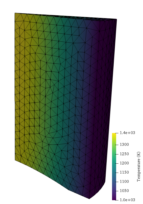
FEniCS implementationWe now consider a portion of nuclear fuel rod (Uranium Dioxide \(\text{UO}_2\)) subject to an external imposed temperature \(T_{ext}=1000\text{ K}\) and uniform volumetric heat source \(r=300 \text{ MW/m}^3\). From the steady state heat balance equation \(\operatorname{div}\mathbf{j} = r\), the variational formulation is now:
\[\begin{equation} F(\widehat{T}) = \int_\Omega \mathbf{j}(T,\nabla T)\cdot\nabla \widehat{T}\,\text{dx} + \int_\Omega r \widehat{T} \,\text{dx}=0 \quad \forall \widehat{T} \end{equation}\]
which fits the general default format of a
MFrontNonlinearProblem: \[\begin{equation}
F(\widehat{u}) = \sum_i \int_\Omega \boldsymbol{\sigma}_i(u)\cdot
\mathbf{g}_i(\widehat{u})\,\text{dx} -L(\widehat{u}) =0 \quad \forall
\widehat{u}
\end{equation}\]
where \((\boldsymbol{\sigma}_i,\mathbf{g}_i)\) are
pairs of dual flux/gradient and here the external loading form \(L\) is given by \(-\int_\Omega r \widehat{T} \,\text{dx}\).
Compared to the previous example, we just add this source term using the
set_loading method. Here we use a quadratic interpolation
for the temperature field and external temperature is imposed on the
surface numbered 12. Finally, we also rely on automatic registration of
the gradient and external state variables as explained in the previous
demo.
from dolfin import *
import mgis.fenics as mf
from time import time

mesh = Mesh()
with XDMFFile("meshes/fuel_rod_mesh.xdmf") as infile:
    infile.read(mesh)
mvc = MeshValueCollection("size_t", mesh, 2)
with XDMFFile("meshes/fuel_rod_mf.xdmf") as infile:
    infile.read(mvc, "facets")
facets = cpp.mesh.MeshFunctionSizet(mesh, mvc)

V = FunctionSpace(mesh, "CG", 2)
T = Function(V, name="Temperature")
T_ = TestFunction(V)
dT = TrialFunction(V)
T0 = Constant(300.)
T.interpolate(T0)

Text = Constant(1e3)
bc = DirichletBC(V, Text, facets, 12)

r = Constant(3e8)

quad_deg = 2
material = mf.MFrontNonlinearMaterial("./src/libBehaviour.so",
                                      "StationaryHeatTransfer")
problem = mf.MFrontNonlinearProblem(T, material, quadrature_degree=quad_deg, bcs=bc)
problem.set_loading(-r*T*dx)
The solve method computing time is monitored:
tic = time()
problem.solve(T.vector())
print("MFront/FEniCS solve time:", time()-tic)
Automatic registration of 'TemperatureGradient' as grad(Temperature).
Automatic registration of 'Temperature' as an external state variable.
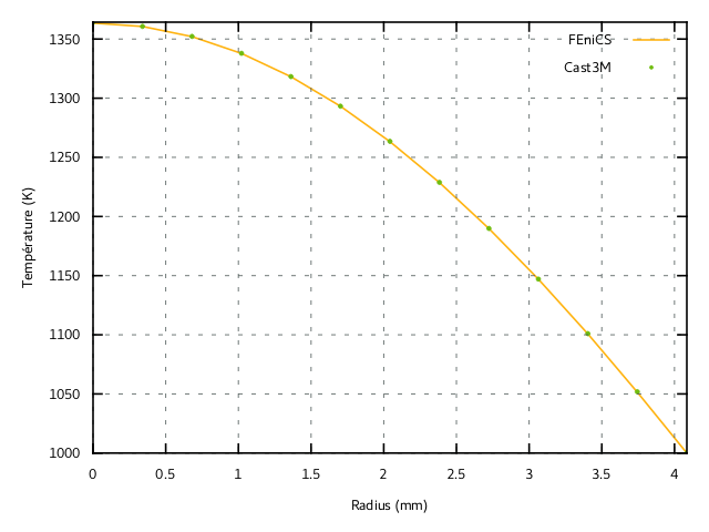
MFront/FEniCS solve time: 53.746278047561646The temperature field along a radial direction along the top surface has been compared with computations using Cast3M finite-element solver. Both solutions agree perfectly, as shown on Figure 1.
FEniCSFor the purpose of performance comparison, we also implement a direct non-linear variational problem with pure UFL expressions. This is possible in the present case since the non-linear heat constitutive law is very simple. Note that we enforce the use of the same quadrature rule degree. The temperature field is also reinterpolated to its previous initial value for a fair comparison between both solution strategies.
A = Constant(material.get_parameter("A"))
B = Constant(material.get_parameter("B"))
j = -1/(A + B*T)*grad(T)
F = (dot(grad(T_), j) + r*T_)*dx(metadata={'quadrature_degree': quad_deg})
J = derivative(F, T, dT)

T.interpolate(T0)
tic = time()
solve(F == 0, T, bc, J=J)
print("Pure FEniCS solve time:", time()-tic)
Pure FEniCS solve time: 49.15058135986328| Mesh type | Quadrature degree | FEniCS/MFront |
Pure FEniCS |
|---|---|---|---|
| coarse | 2 | 1.2 s | 0.8 s |
| coarse | 5 | 2.2 s | 1.0 s |
| fine | 2 | 62.8 s | 58.4 s |
| fine | 5 | 77.0 s | 66.3 s |
We can observe that both methods, relying on the same default Newton
solver, yield the same total iteration counts and residual values. As
regards computing time, the pure FEniCS implementation is
slightly faster as expected. In Table 1, comparison has been made for a
coarse (approx 4 200 cells) and a refined (approx 34 000 cells) mesh
with quadrature degrees equal either to 2 or 5.
The difference is slightly larger for large quadrature degrees, however, the difference is moderate when compared to the total computing time for large scale problems.
Most FE software do not take into account the contribution of \(\dfrac{\partial \mathbf{j}}{\partial T}\)
to the tangent operator. One can easily test this variant by assigning
dj_ddT in the MFront behaviour or change the expression of
the jacobian in the pure FEniCS implementation by:
J = dot(grad(T_), -grad(dT)/(A+B*T))*dx(metadata={'quadrature_degree': quad_deg})In the present case, using this partial tangent operator yields a convergence in 4 iterations instead of 3, giving a computational cost increase by roughly 25%.