This demo is dedicated to the resolution of a finite-strain elastoplastic problem using the logarithmic strain framework proposed in Miehe, Apel, and Lambrecht (2002).
Source files:
- Jupyter notebook: mgis_fenics_finite_strain_elastoplasticity.ipynb
- Python file: mgis_fenics_finite_strain_elastoplasticity.py
- MFront behaviour file: LogarithmicStrainPlasticity.mfront
This framework expresses constitutive relations between the Hencky strain measure \(\boldsymbol{H} = \dfrac{1}{2}\log (\boldsymbol{F}^T\cdot\boldsymbol{F})\) and its dual stress measure \(\boldsymbol{T}\). This approach makes it possible to extend classical small strain constitutive relations to a finite-strain setting. In particular, the total (Hencky) strain can be split additively into many contributions (elastic, plastic, thermal, swelling, etc.). Its trace is also linked with the volume change \(J=\exp(\operatorname{tr}(\boldsymbol{H}))\). As a result, the deformation gradient \(\boldsymbol{F}\) is used for expressing the Hencky strain \(\boldsymbol{H}\), a small-strain constitutive law is then written for the \((\boldsymbol{H},\boldsymbol{T})\)-pair and the dual stress \(\boldsymbol{T}\) is then post-processed to an appropriate stress measure such as the Cauchy stress \(\boldsymbol{\sigma}\) or Piola-Kirchhoff stresses.
MFront implementationThe logarithmic strain framework discussed in the previous paragraph consists merely as a pre-processing and a post-processing stages of the behaviour integration. The pre-processing stage compute the logarithmic strain and its increment and the post-processing stage interprets the stress resulting from the behaviour integration as the dual stress \(\boldsymbol{T}\) and convert it to the Cauchy stress.
MFront provides the @StrainMeasure keyword
that allows to specify which strain measure is used by the behaviour.
When choosing the Hencky strain measure,
MFront automatically generates those pre- and
post-processing stages, allowing the user to focus on the behaviour
integration.
This leads to the following implementation (see the small-strain elastoplasticity example for details about the various implementation available):
@DSL Implicit;
@Behaviour LogarithmicStrainPlasticity;
@Author Thomas Helfer/Jérémy Bleyer;
@Date 07 / 04 / 2020;
@StrainMeasure Hencky;
@Algorithm NewtonRaphson;
@Epsilon 1.e-14;
@Theta 1;
@MaterialProperty stress s0;
s0.setGlossaryName("YieldStress");
@MaterialProperty stress H0;
H0.setEntryName("HardeningSlope");
@Brick StandardElastoViscoPlasticity{
stress_potential : "Hooke" {
young_modulus : 210e9,
poisson_ratio : 0.3
},
inelastic_flow : "Plastic" {
criterion : "Mises",
isotropic_hardening : "Linear" {H : "H0", R0 : "s0"}
}
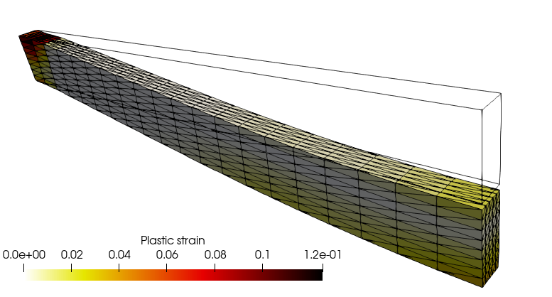
};FEniCS implementationWe define a box mesh representing half of a beam oriented along the \(x\)-direction. The beam will be fully clamped on its left side and symmetry conditions will be imposed on its right extremity. The loading consists of a uniform self-weight.
%matplotlib notebook
import matplotlib.pyplot as plt
from dolfin import *
import mgis.fenics as mf
import numpy as np
import ufl

length, width, height = 1., 0.04, 0.1
nx, ny, nz = 30, 5, 8
mesh = BoxMesh(Point(0, -width/2, -height/2.), Point(length, width/2, height/2.), nx, ny, nz)

V = VectorFunctionSpace(mesh, "CG", 2)
u = Function(V, name="Displacement")

def left(x, on_boundary):
    return near(x[0], 0) and on_boundary
def right(x, on_boundary):
    return near(x[0], length) and on_boundary

bc = [DirichletBC(V, Constant((0.,)*3), left),
      DirichletBC(V.sub(0), Constant(0.), right)]

selfweight = Expression(("0", "0", "-t*qmax"), t=0., qmax = 50e6, degree=0)

file_results = XDMFFile("results/finite_strain_plasticity.xdmf")
file_results.parameters["flush_output"] = True
file_results.parameters["functions_share_mesh"] = True
The MFrontNonlinearMaterial instance is loaded from the
MFront LogarithmicStrainPlasticity behaviour.
This behaviour is a finite-strain behaviour
(material.is_finite_strain=True) which relies on a
kinematic description using the total deformation gradient \(\boldsymbol{F}\). By default, a
MFront behaviour always returns the Cauchy stress as the
stress measure after integration. However, the stress variable dual to
the deformation gradient is the first Piola-Kirchhoff (PK1) stress. An
internal option of the MGIS interface is therefore used in the
finite-strain context to return the PK1 stress as the “flux” associated
to the “gradient” \(\boldsymbol{F}\).
Both quantities are non-symmetric tensors, aranged as a 9-dimensional
vector in 3D following MFront
conventions on tensors.
material = mf.MFrontNonlinearMaterial("./src/libBehaviour.so",
                                      "LogarithmicStrainPlasticity",
                                      material_properties={"YieldStrength": 250e6,
                                                           "HardeningSlope": 1e6})
print(material.behaviour.getBehaviourType())
print(material.behaviour.getKinematic())
print(material.get_gradient_names(), material.get_gradient_sizes())
print(material.get_flux_names(), material.get_flux_sizes())
At this stage, one can retrieve some information about the behaviour:
print(material.behaviour.getBehaviourType())
    StandardFiniteStrainBehaviour
print(material.behaviour.getKinematic())
    F_CAUCHY
print(material.get_gradient_names(), material.get_gradient_sizes())
    ['DeformationGradient'] [9]
print(material.get_flux_names(), material.get_flux_sizes())
    ['FirstPiolaKirchhoffStress'] [9]
The MFrontNonlinearProblem instance must therefore
register the deformation gradient as Identity(3)+grad(u).
This again done automatically since "DeformationGradient"
is a predefined gradient. The following message will be shown upon
calling solve:
Automatic registration of 'DeformationGradient' as I + (grad(Displacement)).The loading is then defined and, as for the small-strain
elastoplasticity example, state variables include the
ElasticStrain and EquivalentPlasticStrain
since the same behaviour is used as in the small-strain case with the
only difference that the total strain is now given by the Hencky strain
measure.
In particular, the ElasticStrain is still a symmetric
tensor (vector of dimension 6). Note that it has not been explicitly
defined as a state variable in the MFront behaviour file
since this is done automatically when using the
IsotropicPlasticMisesFlow domain specific language.
Finally, we setup a few parameters of the Newton non-linear solver.
problem = mf.MFrontNonlinearProblem(u, material, bcs=bc)
problem.set_loading(dot(selfweight, u)*dx)

epsel = problem.get_state_variable("ElasticStrain")

prm = problem.solver.parameters
prm["absolute_tolerance"] = 1e-6
prm["relative_tolerance"] = 1e-6
prm["linear_solver"] = "mumps"
Information about how the elastic strain is stored can be retrieved as follows:
print("'ElasticStrain' shape:", ufl.shape(epsel))
    'ElasticStrain' shape: (6,)
During the load incrementation, we monitor the evolution of the vertical downwards displacement at the middle of the right extremity.
Nincr = 30
load_steps = np.linspace(0., 1., Nincr+1)
results = np.zeros((Nincr+1, 3))
for (i, t) in enumerate(load_steps[1:]):
    selfweight.t = t
    print("Increment ", i+1)
    problem.solve(u.vector())
    p0 = problem.get_state_variable("EquivalentPlasticStrain", project_on=("DG", 0))

    file_results.write(u, t)
    file_results.write(p0, t)

    results[i+1, 0] = -u(length, 0, 0)[2]
    results[i+1, 1] = t
This simulation is a bit heavy to run so we suggest running it in parallel:
mpirun -np 4 python3 finite_strain_elastoplasticity.pyThe load-displacement curve exhibits a classical elastoplastic behaviour rapidly followed by a stiffening behaviour due to membrane catenary effects.
plt.figure()
plt.plot(results[:, 0], results[:, 1], "-o")
plt.xlabel("Displacement")
plt.ylabel("Load");
<IPython.core.display.Javascript object>