Phase-field approach to brittle fracture

The present demo illustrates how multi-physics problems can be coupled and solved in a staggered fashion. This problematic is illustrated on a phase-field approach to brittle fracture in which two different mechanical problems are involved:

The problem is that of a stiff circular inclusion embedded in a square plate under imposed vertical displacement on its top surface, see Bourdin, Francfort, and Marigo (2000). Zero Dirichlet boundary conditions will be enforced for the damage field on the inclusion boundary.

Introduction on phase-field approaches to brittle fracture

The phase-field approach to brittle fracture originates from the mathematical regularization of Francfort & Marigo variational approach of fracture (see Francfort and Marigo (1998)). Following mathematical works of Ambrosio and Tortorelli (1990), the regularization proposed by Bourdin, Francfort, and Marigo (2000) relies on the following total energy $\mathcal{E}(u, d) = \mathcal{E}_\text{pot}(u,d)+\mathcal{E}_\text{frac}(d)$ where the potential and fracture energies respectively read as:

\[ \begin{aligned} \mathcal{E}_\text{pot}(u,d) &= \int_\Omega g(d)\dfrac{1}{2}\boldsymbol{\varepsilon}:\mathbb{C}:\boldsymbol{\varepsilon}\,\text{dx}- W_{ext}(u) \\ \mathcal{E}_\text{frac}(d) &= \dfrac{G_c}{c_w} \int_{\Omega}\left( \frac{w(d)}{\ell_0} + \ell_0 \|\nabla d\|^2 \right)\,\text{dx} \end{aligned} \]

Solutions to the quasi-static evolution at discrete time steps $(u_n,d_n)$ are obtained from a global energy minimum principle on both variables with an additional irreversibility constraint $d_n\geq d_{n-1}$ for the damage variable.

This original formulation does not distinguish between tensile and compressive stress states, yielding spurious crack formation in compressive regions. A commonly used remedy consists in splitting the energy density $\psi$ into a positive (associated with tension states) and negative (compressive states) part and apply the degradation function only on the positive part i.e.:

\[ \mathcal{E}_{pot}(u,d) = \int_\Omega \left(g(d)\psi^+(\boldsymbol{\varepsilon})+\psi^-(\boldsymbol{\varepsilon})\right) \,\text{dx}- W_{ext}(u) \]

Different choices of this splitting exist and we use in this demo the volumetric/deviatoric splitting introduced in Amor, Marigo, and Maurini (2009):

\[ \begin{aligned} \psi^+(\boldsymbol{\varepsilon}) &= \dfrac{1}{2}\kappa \langle \operatorname{tr}(\boldsymbol{\varepsilon})\rangle_+^2 + \mu \operatorname{dev}(\boldsymbol{\varepsilon}):\operatorname{dev}(\boldsymbol{\varepsilon})\\ \psi^-(\boldsymbol{\varepsilon}) &= \dfrac{1}{2}\kappa \langle \operatorname{tr}(\boldsymbol{\varepsilon})\rangle_-^2 \end{aligned} \]

where $\langle \star \rangle_\pm$ denotes the positive/negative part function, $\operatorname{dev}$ is the deviatoric operator and $\kappa=\lambda+\dfrac{2}{3}\mu$ stands for the compression modulus. Note that we also provide an implementation of the spectral splitting introduced by Miehe, Hofacker, and Welschinger (2010) in the PhaseFieldDisplacementSpectralSplit.mfront file

A classical choice for the degradation function is $g(d)=(1-d)^2 + k_\text{res}$ where $k_\text{res} \ll 1$ is a residual stiffness avoiding singular stiffness in the fully damaged state. As regards the fracture energy density, two choices originating from the work of Ambrosio and Tortorelli (AT) are widely used, namely:

\[ \begin{aligned} \text{AT2 model:} \quad & w(d) = d^2, \quad c_w=2\\ \text{AT1 model:} \quad & w(d) = d, \quad c_w=\dfrac{8}{3} \end{aligned} \]

in which the constant $c_w$ is chosen so that analytical localized solution profiles correspond to a dissipated precisely equal to $G_c$.

Numerical resolution techniques

A classical approach for computing the solution at load increment $n$ is to resort to a so-called alternate minimization scheme which involves the following steps embedded in an iterative procedure:

\[\begin{align} u^k &= \mathrm{arg min}_u \mathcal{E}(u, d^{k-1}) \tag{$u$-problem}\\ d^k &= \mathrm{arg min}_{d \text{ s.t. } d_{n-1} \leq d} \mathcal{E}(u^k, d) \tag{$d$-problem} \end{align}\]

The first step ($u$-problem) of this staggered solution scheme therefore involves solving the following non-linear mechanical problem at fixed damage:

\[ \textrm{Find } u\in V_u \text{ s.t. } \int_\Omega \boldsymbol{\sigma}(u,d_{k-1}):\operatorname{sym}\nabla \widehat{u} \,\text{dx} = W_{ext}(\widehat{u}) \quad \forall \widehat{u}\in V_u \]

with $\boldsymbol{\sigma}(u,d)=g(d)\dfrac{\partial \psi^+}{\partial \boldsymbol{\varepsilon}}(u)+\dfrac{\partial \psi^-}{\partial \boldsymbol{\varepsilon}}(u)$.

The second step ($d$-problem) amounts to solving a variational inequality problem due to the presence of the irreversibility constraint $d_{n-1} \leq d$. A simple way of enforcing, implicitly, this irreversibility constraint has been proposed in Miehe, Hofacker, and Welschinger (2010) by resorting to a so-called history function which correspond to the maximal value of the tensile energy density $\psi^+$ over the past loading history:

Technically, the irreversibility constraint is dropped and the current tensile energy $\psi^+$ is substituted by $H$ in the $d$-problem. The optimality condition therefore yields the following variational problem:

\[ \textrm{Find } d\in V_d \text{ s.t. } \int_\Omega \left(g'(d)H\widehat{d}+\dfrac{G_c}{\ell_0c_w}\left(w'(d)\widehat{d} + 2\ell_0^2 \nabla d \cdot \nabla \widehat{d}\right)\right) \,\text{dx} = 0 \quad \forall \widehat{d}\in V_d \]

MFront behaviour for the displacement problem

For the retained choice of models, the stress/strain constitutive equation at fixed damage reads as:

\[ \boldsymbol{\sigma}(\boldsymbol{\varepsilon},d)=((1-d)^2+k_\text{res})\left(\kappa \langle \operatorname{tr}(\boldsymbol{\varepsilon})\rangle_+\textbf{I} + 2\mu \operatorname{dev}(\boldsymbol{\varepsilon})\right)+\kappa \langle \operatorname{tr}(\boldsymbol{\varepsilon})\rangle_- \textbf{I} \]

The stress is here explicitly computed from the strain (as in the non-linear heat transfer demo) so that we use the DefaultDSL. Material properties are defined, the history function and positive energy density are decleared as (internal) state variables whereas the damage field is declared as an external state variable.

@DSL DefaultDSL;
@Author Jérémy Bleyer, Thomas Helfer;
@Date 08 / 04 / 2020;
@Behaviour PhaseFieldDisplacementDeviatoricSplit;

@MaterialProperty stress Yg;
Yg.setGlossaryName("YoungModulus");
@MaterialProperty real ν;
ν.setGlossaryName("PoissonRatio");

@Parameter real kres = 1e-6;
kres.setEntryName("ResidualStiffness");

@StateVariable real H;
H.setEntryName("HistoryFunction");

@StateVariable real Ψ₊;
Ψ₊.setEntryName("PositiveEnergyDensity");

@ExternalStateVariable real d;
d.setGlossaryName("Damage");

We now write the behaviour and provide consistent tangent operators for the problem at fixed damage i.e. the tangent operator is actually the secant operator for the coupled $(u,d)$ problem.

@ProvidesSymmetricTangentOperator;
@Integrator {
  // update the damage
  const auto d_ = d + dd;
  // lame coefficients
  const auto λ = computeLambda(Yg, ν);
  const auto μ = computeMu(Yg, ν);
  // compression modulus
  const auto κ = λ + 2 / 3 ⋅ μ;
  // computation of the stress, positive energy density and consistent
  // tangent operator
  const auto ε = eval(eto + deto);
  const auto tr = trace(ε);
  const auto εᵈ = deviator(ε);
  // energy density
  const auto tr_p = max(tr, strain(0));
  const auto tr_n = tr - tr_p;
  Ψ₊ = (κ / 2) ⋅ (tr_p) ⋅ (tr_p) + μ ⋅ (εᵈ | εᵈ);
  // history function
  H = max(H, Ψ₊);
  // degradation function
  const auto gᵈ = (1 - d_) ⋅ (1 - d_) + kres; 
  // stress
  σ = κ ⋅ (gᵈ ⋅ tr_p + tr_n) ⋅ I₂ + 2 ⋅ μ ⋅ gᵈ ⋅ εᵈ;
  // consistent tangent operator (secant one here)
  if (computeTangentOperator_) {
    static_cast<void>(smt);
    if (tr >= 0) {
      ∂σ∕∂Δεᵗᵒ = gᵈ ⋅ (κ ⋅ (I₂ ⊗ I₂) + 2 ⋅ μ ⋅ Stensor4::K());
    } else {
      ∂σ∕∂Δεᵗᵒ = κ ⋅ (I₂ ⊗ I₂) + gᵈ ⋅ 2 ⋅ μ ⋅  Stensor4::K();
    }
  }
} // end of @Integrator

note that we used Stensor4::K() in the above definition, which correspond to $\mathbb{K} = \mathbb{I}-\dfrac{1}{3}\mathbf{I}\otimes\mathbf{I}$, the projection operator on the deviatoric space $\mathbb{K}:\boldsymbol{\varepsilon}= \operatorname{dev}(\boldsymbol{\varepsilon})$.

@InternalEnergy {
  const auto gᵈ = ((1 - d) ⋅ (1 - d)) + kres;
  Psi_s = gᵈ ⋅ Ψ₊;
}

MFront behaviour for the damage problem

The damage problem variational form using the history function approach for the AT2 model writes:

\[ \textrm{Find } d\in V_d \text{ s.t. } \int_\Omega \left(\dfrac{G_c}{\ell_0}\left(\ell_0^2 \nabla d \cdot \nabla \widehat{d} + d \widehat{d}\right) - 2H(1-d)\widehat{d}\right) \,\text{dx} = 0 \quad \forall \widehat{d}\in V_d \]

which can therefore be rewritten as follows to fit the standard format using pairs of flux/gradient variables:

\[ \textrm{Find } d\in V_d \text{ s.t. } \int_\Omega (\mathbf{q}\cdot \nabla \widehat{d} + Y\widehat{d})\,\text{dx} = 0 \quad \forall \widehat{d}\in V_d \]

where $\mathbf{q} = G_c \ell_0 \nabla d$ is the dual “flux”-like variable associated with the damage gradient $\mathbf{g} =\nabla d$ and $Y=\left(\dfrac{G_c}{\ell_0}+2H\right)d-2H$ is the dual “flux”-like variable associated with the damage itself, interpreted (up to a change of sign) as an energy release rate.

@DSL DefaultGenericBehaviour;
@Behaviour PhaseFieldDamage;
@Author Jérémy Bleyer;
@Date 07 / 04 / 2020;

@Gradient real d;
d.setGlossaryName("Damage");
@Flux real Y;
Y.setEntryName("EnergyRelease");

@Gradient TVector g;
g.setEntryName("DamageGradient");
@Flux TVector q;
q.setEntryName("DualDamageGradient");

@TangentOperatorBlock ∂q∕∂Δg;
@AdditionalTangentOperatorBlock ∂Y∕∂Δd;

where the pairs $(Y,d)$ and $(\mathbf{q},\mathbf{g})$ of dual variables have been defined using the DefaultGenericBehaviour and the corresponding required tangent operator blocks ∂q∕∂Δg and ∂Y∕∂Δd have been defined.

Material properties $G_c$ and $\ell_0$ are now defined and we declare the history function $H$ as an external state variable.

@MaterialProperty real l₀;
l₀.setEntryName("RegularizationLength");
@MaterialProperty real Gc;
Gc.setEntryName("FractureEnergy");

@ExternalStateVariable real H;
H.setEntryName("HistoryFunction");

Finally, the integrator writes the linear behaviour and defines the expressions for the tangent operator blocks and we also compute the dissipated fracture energy density:

@ProvidesTangentOperator;
@Integrator {
  // remove useless warnings, as we always compute the tangent operator
  static_cast<void>(computeTangentOperator_);
  ∂q∕∂Δg = Gc*l₀* tmatrix<N, N, real>::Id();
  ∂Y∕∂Δd = Gc/l₀+2*H;
  q = Gc*l₀*(g+Δg);
  Y = ∂Y∕∂Δd ⋅ (d+Δd)-2*H;
}

@DissipatedEnergy{
Psi_d = Gc/2/l₀*(d*d + l₀*l₀*(g|g));
}

FEniCS implementation

from dolfin import *
from mshr import *
import mgis.fenics as mf
import numpy as np
import matplotlib.pyplot as plt
from IPython.display import clear_output

N = 100
domain = Rectangle(Point(0, 0), Point(1, 1)) - Circle(Point(0.5, 0.5), 0.2, 40)
mesh = generate_mesh(domain, N)

Vu = VectorFunctionSpace(mesh, "CG", 1)
u  = Function(Vu, name="Displacement")

def top(x, on_boundary):
    return near(x[1], 1) and on_boundary
def internal(x, on_boundary):
    return near((x[0]-0.5)**2+(x[1]-0.5)**2, 0.2**2, 0.05) and on_boundary
Uimp = Expression(("0", "t"), t=1, degree=0)
bcu = [DirichletBC(Vu, Constant((0, 0)), internal),
       DirichletBC(Vu, Uimp, top)]
v = Function(Vu)
bcu[1].apply(v.vector())

Vd = FunctionSpace(mesh, "CG", 1)
d = Function(Vd, name="Damage")
dold = Function(Vd, name="Previous damage")
bcd = DirichletBC(Vd, Constant(0.), internal)

We now define the displacement $u$-problem by loading the PhaseFieldDisplacement behaviour. Since the damage variable has been declared as an external state variable for this problem, we must register it with the damage field d. We also retrieve the HistoryFunction internal state variable H which will then be used as an external state variable for the damage problem. We finally recall that automatic registration of the strain is used here.

E, nu = 200, 0.2
material_u = mf.MFrontNonlinearMaterial("./src/libBehaviour.so",
                                      "PhaseFieldDisplacementDeviatoricSplit",
                                      hypothesis="plane_strain",
                                      material_properties={"YoungModulus": E,
                                                            "PoissonRatio": nu})
problem_u = mf.MFrontNonlinearProblem(u, material_u, quadrature_degree=0, bcs=bcu)
problem_u.register_external_state_variable("Damage", d)
H = problem_u.get_state_variable("HistoryFunction")
problem_u.solver.parameters["report"] = False

Similarly, the damage problem is defined from the PhaseFieldDamage behaviour. The latter is a generalized behaviour which involves two gradients (as discussed in the corresponding section) which must be registered with their corresponding UFL representations. As mentioned before, for this behaviour HistoryFunction is an external state variable which is now registered as being H.

Gc, l0 = 1., 0.02
material_d = mf.MFrontNonlinearMaterial("./src/libBehaviour.so",
                                      "PhaseFieldDamage",
                                      hypothesis="plane_strain",
                                      material_properties={"RegularizationLength": l0,
                                                            "FractureEnergy": Gc})

problem_d = mf.MFrontNonlinearProblem(d, material_d, quadrature_degree=0, bcs=bcd)
problem_d.register_gradient("Damage", d)
problem_d.register_gradient("DamageGradient", grad(d))
problem_d.register_external_state_variable("HistoryFunction", H)
problem_d.solver.parameters["report"] = False

We now implement the load-stepping procedure and, for each load step, the alternate minimization algorithm between the $u$-problem and the $d$-problem. The alternate minimization iterations are stopped when $|d-d_{old}|_ $ between two consecutive damage fields.

After convergence of an alternate minimization step, we compute the vertical force acting on the top surface. For this purpose, we previously defined a function v with a vertical component equal to 1 on the top boundary and zero everywhere. The action of the residual form in this field is precisely the resulting vertical force of the imposed boundary conditions. We also compute the total stored and dissipated energy. The former has been defined in PhaseFieldDisplacement.mfront and the second in PhaseFieldDamage.mfront.

tol, Nitermax = 1e-3, 500
loading = np.concatenate((np.linspace(0, 70e-3, 6),
                          np.linspace(70e-3, 125e-3, 26)[1:]))
N = loading.shape[0]
results = np.zeros((N, 3))
for (i, t) in enumerate(loading[1:]):
    print("Time step:", i+1)
    Uimp.t = t
    # Start alternate minimization
    res = 1.
    j = 1
    while res > tol and j < Nitermax:
        # Solve displacement u-problem
        problem_u.solve(u.vector())
        # Solve damage d-problem
        dval_old = d.vector().get_local()
        problem_d.solve(d.vector())
        # Residual on damage increment
        dval = d.vector().get_local()
        res = np.max(dval - dval_old)
        
        print("   Iteration {}: {}".format(j, res))
        j += 1

    results[i+1, 0] = assemble(action(problem_u.residual, v))
    results[i+1, 1] = problem_u.get_stored_energy()
    results[i+1, 2] = problem_d.get_dissipated_energy()
    
    clear_output(wait = True)
    plt.figure()
    p=plot(d, vmin=0, vmax=1)
    plt.colorbar(p)
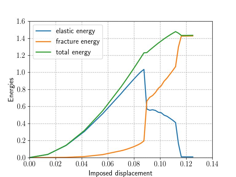
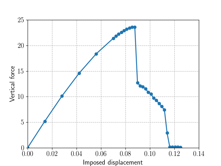
    plt.savefig("./results/phase_field_{:04d}.png".format(i), dpi=400)

Load-displacement and energy evolution curves show that there is a phase of brutal crack nucleation followed by a more stable crack propagation phase towards the plate boundaries. The solution vertical symmetry is lost in the last load steps when approaching the plate boundaries as already mentioned in Bourdin, Francfort, and Marigo (2000).

%matplotlib notebook

plt.figure()
plt.plot(loading, results[:, 0], "-o")
plt.xlabel("Imposed displacement")
plt.ylabel("Vertical force")
plt.show()

plt.figure()
plt.plot(loading, results[:, 1], label="elastic energy")
plt.plot(loading, results[:, 2], label="fracture energy")
plt.plot(loading, results[:, 1] + results[:, 2], label="total energy")
plt.xlabel("Imposed displacement")
plt.ylabel("Energies")
plt.legend()
plt.show()

References

Ambrosio, Luigi, and Vincenzo Maria Tortorelli. 1990. “Approximation of Functional Depending on Jumps by Elliptic Functional via t-Convergence.” Communications on Pure and Applied Mathematics 43 (8): 999–1036.

Amor, Hanen, Jean-Jacques Marigo, and Corrado Maurini. 2009. “Regularized Formulation of the Variational Brittle Fracture with Unilateral Contact: Numerical Experiments.” Journal of the Mechanics and Physics of Solids 57 (8): 1209–29.

Bourdin, Blaise, Gilles A Francfort, and Jean-Jacques Marigo. 2000. “Numerical Experiments in Revisited Brittle Fracture.” Journal of the Mechanics and Physics of Solids 48 (4): 797–826.

Francfort, Gilles A, and J-J Marigo. 1998. “Revisiting Brittle Fracture as an Energy Minimization Problem.” Journal of the Mechanics and Physics of Solids 46 (8): 1319–42.

Miehe, Christian, Martina Hofacker, and Fabian Welschinger. 2010. “A Phase Field Model for Rate-Independent Crack Propagation: Robust Algorithmic Implementation Based on Operator Splits.” Computer Methods in Applied Mechanics and Engineering 199 (45-48): 2765–78.

Pham, Kim, Hanen Amor, Jean-Jacques Marigo, and Corrado Maurini. 2011. “Gradient Damage Models and Their Use to Approximate Brittle Fracture.” International Journal of Damage Mechanics 20 (4): 618–52.