This demo explores the full capability of MFront’s
recent extension to handling generalized behaviours, namely involving
different pairs of fluxes and gradients, as well as FEniCS
versatility to solve generic PDEs.
This will be illustrated on a generalized continuum model called multiphase model in the context of fiber-reinforced materials (Bleyer 2018).
Source files:
- Jupyter notebook: mgis_fenics_multiphase_model.ipynb
- Python file: mgis_fenics_multiphase_model.py
- MFront behaviour file: MultiphaseModel.mfront
The multiphase model is a higher-grade (i.e. with enhanced kinematics) generalized continuum which represents a biphasic material (the main application being fiber-reinforced materials) by a superposition of two phases (say matrix and fiber phases), each possessing their own kinematics and in mutual interaction. Each phase kinematics is described by a displacement field \(\boldsymbol{U}^1\) and \(\boldsymbol{U}^2\) for the matrix and fiber phase respectively.
In the present case, each phase is a standard Cauchy continuum but other variants, including fiber bending effects for instance, exist, see De Buhan, Bleyer, and Hassen (2017) for more details.
Generalized strains: infinitesimal strain in each phase \(\boldsymbol{\varepsilon}^j=\nabla^s \boldsymbol{U}^j\) and relative displacement between both phases \(\boldsymbol{V}= \boldsymbol{U}^2-\boldsymbol{U}^1\)
Generalized stresses: partial stress \(\boldsymbol{\sigma}^j\) in both phases and interaction force \(\boldsymbol{I}\) (exerted by phase 2 over phase 1)
Equilibrium equations:
\[\begin{align} \operatorname{div}\boldsymbol{\sigma}^1 +\rho_1F + \boldsymbol{I}&= 0 \label{multiphase-eq1}\\ \operatorname{div}\boldsymbol{\sigma}^2 + \rho_2F - \boldsymbol{I}&= 0 \label{multiphase-eq2} \end{align}\]
\[\begin{align} \boldsymbol{\sigma}^1\cdot\boldsymbol{t}&= \boldsymbol{n}^1 \text{ on }\partial \Omega_{T} \\ \boldsymbol{\sigma}^2\cdot\boldsymbol{t}&= \boldsymbol{n}^2 \text{ on } \partial \Omega_{T} \end{align}\]
\[\begin{equation} w_{\text{def}} = \boldsymbol{\sigma}^1:\boldsymbol{\varepsilon}^1 + \boldsymbol{\sigma}^2:\boldsymbol{\varepsilon}^2+ \boldsymbol{I}\cdot\boldsymbol{V} \end{equation}\]
\[\begin{align} \boldsymbol{\sigma}^1 &= \dfrac{\partial \psi}{\partial \boldsymbol{\varepsilon}^1}(\boldsymbol{\varepsilon}^1,\boldsymbol{\varepsilon}^2,\boldsymbol{V}) \\ \boldsymbol{\sigma}^2 &= \dfrac{\partial \psi}{\partial \boldsymbol{\varepsilon}^2}(\boldsymbol{\varepsilon}^1,\boldsymbol{\varepsilon}^2,\boldsymbol{V})\\ \boldsymbol{I}&= \dfrac{\partial \psi}{\partial \boldsymbol{V}}(\boldsymbol{\varepsilon}^1,\boldsymbol{\varepsilon}^2,\boldsymbol{V}) \end{align}\]
which will be particularized for the present demo to the following elastic behaviour:
\[\begin{align*} \boldsymbol{\sigma}^1 &= \mathbb{D}^{11}:\boldsymbol{\varepsilon}^1+\mathbb{D}^{12}:\boldsymbol{\varepsilon}^2\\ \boldsymbol{\sigma}^2 &= (\mathbb{D}^{12}){}^\text{T}:\boldsymbol{\varepsilon}^1+\mathbb{D}^{22}:\boldsymbol{\varepsilon}^2\\ \boldsymbol{I}&= \boldsymbol{\kappa}\cdot \boldsymbol{V} \end{align*}\] in which \(\mathbb{D}^{ij}\) are partial stiffness tensors and \(\kappa\) can be seen as an interaction stiffness between both phases.
MFront implementationThe MFront implementation expands upon the detailed
MFront implementation of the stationnary heat transfer demo.
Again, the DefaultGenericBehaviour is used here and specify
that the following implementation will only handle the 2D plane strain
case.
@DSL DefaultGenericBehaviour;
@Behaviour MultiphaseModel;
@Author Jeremy Bleyer;
@Date 04/04/2020;

@ModellingHypotheses {PlaneStrain};The three pairs of generalized flux/gradient of the multiphase model are then defined, namely \((\boldsymbol{\sigma}^1,\boldsymbol{\varepsilon}^1)\), \((\boldsymbol{\sigma}^2,\boldsymbol{\varepsilon}^2)\) and \((\boldsymbol{I},\boldsymbol{V})\):
@Gradient StrainStensor e₁;
e₁.setEntryName("MatrixStrain");
@Flux StressStensor σ₁;
σ₁.setEntryName("MatrixStress");

@Gradient StrainStensor e₂;
e₂.setEntryName("FiberStrain");
@Flux StressStensor σ₂;
σ₂.setEntryName("FiberStress");

@Gradient TVector V;
V.setEntryName("RelativeDisplacement");
@Flux TVector I;
I.setEntryName("InteractionForce");
We now declare the various tangent operator blocks which will be needed to express the generalized tangent operator. Of the nine possible blocks, only 5 are needed here since the partial stresses do not depend on the relative displacement and, similarly, the interaction force does not depend on the phase strains:
@TangentOperatorBlocks{∂σ₁∕∂Δe₁,∂σ₁∕∂Δe₂,∂σ₂∕∂Δe₁,∂σ₂∕∂Δe₂,∂I∕∂ΔV};We consider the case of a 2D plane strain bilayered material made of isotropic materials for both the matrix and fiber phases. In addition to the four material constants need for both constituents, the volume fraction of both phases (here we ask for the volume fraction \(\rho\) of the fiber phase) and the size \(s\) of the material unit cell (i.e. the spacing between two consecutive matrix layers for instance) are the two other parameters characterizing the multiphase elastic model.
@MaterialProperty stress Y1;
Y1.setEntryName("MatrixYoungModulus");
@MaterialProperty real nu1;
nu1.setEntryName("MatrixPoissonRatio");
@MaterialProperty stress Y2;
Y2.setEntryName("FiberYoungModulus");
@MaterialProperty real nu2;
nu2.setEntryName("FiberPoissonRatio");
@MaterialProperty real ρ;
ρ.setEntryName("FiberVolumeFraction");
@MaterialProperty real s;
s.setEntryName("Size");It has been shown in Bleyer (2018) that, for materials made of two constituents, the partial stiffness tensors \(\mathbb{D}^{ij}\) can be expressed as functions of the material individual stiffness \(\mathbb{C}^1,\mathbb{C}^2\) and the macroscopic stiffness \(\mathbb{C}^{hom}\) of the composite (obtained from classical homogenization theory) as follows:
\[\begin{align*} \mathbb{D}^{11} &= \phi_1\mathbb{C}^1-\mathbb{C}^1:[\![\mathbb{C}]\!]^{-1}:\Delta\mathbb{C}:[\![\mathbb{C}]\!]^{-1}:\mathbb{C}^1\\ \mathbb{D}^{22} &= \phi_2\mathbb{C}^2-\mathbb{C}^2:[\![\mathbb{C}]\!]^{-1}:\Delta\mathbb{C}:[\![\mathbb{C}]\!]^{-1}:\mathbb{C}^2\\ \mathbb{D}^{12} &= \mathbb{C}^1:[\![\mathbb{C}]\!]^{-1}:\Delta\mathbb{C}:[\![\mathbb{C}]\!]^{-1}:\mathbb{C}^2 \end{align*}\]
with \(\phi_1=1-\rho\), \(\phi_2 = \rho\) are the phases volume fractions, \([\![\mathbb{C}]\!]=\mathbb{C}^2-\mathbb{C}^1\) and \(\Delta\mathbb{C}= \phi_1\mathbb{C}^1+\phi_2\mathbb{C}^2-\mathbb{C}^{hom}\). They satisfy the following property \(\mathbb{D}^{11}+\mathbb{D}^{22}+\mathbb{D}^{12}+(\mathbb{D}^{21}){}^\text{T}=\mathbb{C}^{hom}\).
In the present case of a 2D bilayered material made of isotropic constituents, the macroscopic stiffness is given by De Buhan, Bleyer, and Hassen (2017):
\[\begin{equation} \mathbb{C}^{hom} = \begin{bmatrix} \left\langle E_\text{oe}\right\rangle - \left\langle\lambda^2/E_\text{oe}\right\rangle+\left\langle\lambda/E_\text{oe}\right\rangle^2/\left\langle 1/E_\text{oe}\right\rangle & \left\langle\lambda/E_\text{oe}\right\rangle/\left\langle 1/E_\text{oe}\right\rangle & \left\langle\lambda/E_\text{oe}\right\rangle/\left\langle 1/E_\text{oe}\right\rangle & 0 \\ \left\langle\lambda/E_\text{oe}\right\rangle/\left\langle 1/E_\text{oe}\right\rangle & 1/\left\langle 1/E_\text{oe}\right\rangle & \left\langle\lambda\right\rangle & 0 \\ \left\langle\lambda/E_\text{oe}\right\rangle/\left\langle 1/E_\text{oe}\right\rangle & \left\langle\lambda\right\rangle & \left\langle E_\text{oe}\right\rangle & 0 \\ 0 & 0 & 0 & 2/\left\langle 1/\mu\right\rangle \end{bmatrix}_{(xx,yy,zz,xy)} \end{equation}\]
where \(\left\langle\star\right\rangle=\phi_1\star_1+\phi_2\star_2\) denotes the averaging operator and \(E_\text{oe}=\lambda+2\mu\) is the oedometric modulus.
As regards the interaction stiffness tensor, it is obtained from the resolution of an auxiliary homogenization problem formulated on the heterogeneous material unit cell. In the present case, one obtains Bleyer (2018):
\[\begin{equation} \boldsymbol{\kappa}= \begin{bmatrix} \dfrac{12}{\left\langle\mu\right\rangle s^2} & 0 \\ 0 & \dfrac{12}{\left\langle E_\text{oe}\right\rangle s^2} \end{bmatrix}_{(x,y)} \end{equation}\]
These relations are all implemented in the behaviour
@Integrator which also defines the required tangent blocks.
MFront linear algebra on fourth-order tensor makes the
implementation very easy and Unicode support provides much more readable
code.
@ProvidesTangentOperator;
@Integrator {
  // remove useless warnings, as we always compute the tangent operator
  static_cast<void>(computeTangentOperator_);

  const auto λ₁ = computeLambda(Y1,nu1);
  const auto μ₁ = computeMu(Y1,nu1);
  const auto λ₂ = computeLambda(Y2,nu2);
  const auto μ₂ = computeMu(Y2,nu2);
  const auto Eₒₑ¹ = λ₁+2*μ₁;
  const auto Eₒₑ² = λ₂+2*μ₂;
  const auto Eₒₑ = (1-ρ)*Eₒₑ¹ + ρ*Eₒₑ²;
  const auto iEₒₑ = (1-ρ)/Eₒₑ¹ + ρ/Eₒₑ²;
  const auto λ = (1-ρ)*λ₁ + ρ*λ₂;
  const auto λiEₒₑ = (1-ρ)*λ₁/Eₒₑ¹ + ρ*λ₂/Eₒₑ²;
  const auto λ2iEₒₑ = (1-ρ)*λ₁*λ₁/Eₒₑ¹ + ρ*λ₂*λ₂/Eₒₑ²;
  const auto iμ = (1-ρ)/μ₁ + ρ/μ₂;
  const auto C₁₁₁₁ʰᵒᵐ = Eₒₑ - λ2iEₒₑ + λiEₒₑ*λiEₒₑ/iEₒₑ;
  const auto C₁₁₂₂ʰᵒᵐ = λiEₒₑ/iEₒₑ;
  const Stensor4 Cʰᵒᵐ = {
      C₁₁₁₁ʰᵒᵐ , C₁₁₂₂ʰᵒᵐ, C₁₁₂₂ʰᵒᵐ, 0., //
      C₁₁₂₂ʰᵒᵐ, 1/iEₒₑ, λ, 0., //
      C₁₁₂₂ʰᵒᵐ, λ, Eₒₑ, 0., //
      0., 0., 0., 2/iμ
  };
  const auto C¹ = λ₁ ⋅ (I₂ ⊗ I₂) + 2 ⋅ μ₁ ⋅ I₄;
  const auto C² = λ₂ ⋅ (I₂⊗I₂) + 2 ⋅ μ₂ ⋅ I₄;
  const auto iΔC = invert(C²-C¹);
  const auto Cᵃᵛᵍ = (1-ρ)⋅C¹ + ρ⋅C²;
  const auto H = iΔC ⋅ (Cᵃᵛᵍ-Cʰᵒᵐ) ⋅ iΔC;
  const auto D¹¹ = (1-ρ)⋅C¹-(C¹ ⋅ H ⋅ C¹);
  const auto D²² = ρ⋅C²-(C² ⋅ H ⋅ C²);
  const auto D¹² = C¹ ⋅ H ⋅ C²;
  ∂σ₁∕∂Δe₁ = D¹¹;
  ∂σ₁∕∂Δe₂ = D¹²;
  ∂σ₂∕∂Δe₁ = transpose(D¹²);
  ∂σ₂∕∂Δe₂ = D²²;
  σ₁ = ∂σ₁∕∂Δe₁ ⋅ (e₁ + Δe₁) + ∂σ₁∕∂Δe₂ ⋅ (e₂ + Δe₂);
  σ₂ = ∂σ₂∕∂Δe₁ ⋅ (e₁ + Δe₁) + ∂σ₂∕∂Δe₂ ⋅ (e₂ + Δe₂);

  const auto κʰ = 12/iμ/s/s; // horizontal interaction stiffness
  const auto κᵛ = 12/iEₒₑ/s/s; // vertical interaction stiffness
  const tmatrix<N, N, real> κ = {
      κʰ, 0.,
      0., κᵛ
  };
  ∂I∕∂ΔV = κ;
  I = κ ⋅ (V + ΔV);
}
FEniCS implementationWe consider a rectangular domain with a standard \(P_1\) Lagrange interpolation for both
displacement fields \(\boldsymbol{U}^1,\boldsymbol{U}^2\). The
total mixed function space V is therefore made of two
vectorial \(P_1\) Lagrange elementary
spaces. The same boundary conditions will be applied for both phases:
fixed vertical displacement on the bottom boundary, imposed vertical
displacement on the top boundary and fixed horizontal displacement on
the left boundary. The considered problem corresponds to the pure
compression of a multilayered block, an example treated in the
previously mentioned references.
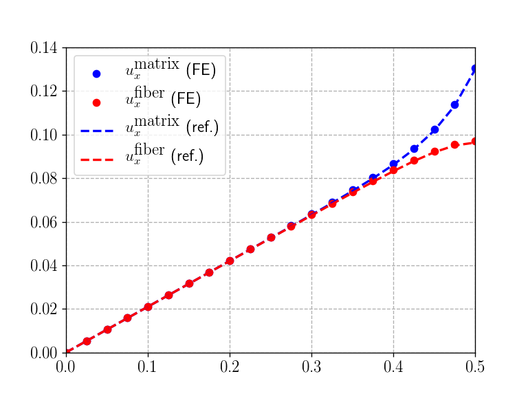
In such a problem, both phase strains are uniform along the vertical direction solution but vary along the horizontal direction due to a boundary layer effect appearing near the right free-edge. Such a feature cannot be captured by a classical Cauchy continuum but is well reproduced by the multiphase model.
%matplotlib notebook
import matplotlib.pyplot as plt
from dolfin import *
import mgis.fenics as mf
import numpy as np
from ufl import diag

width = 0.5
height = 1.
mesh = RectangleMesh(Point(0., 0.), Point(width, height), 100, 100)

Ve = VectorElement("CG", mesh.ufl_cell(), 1)
V = FunctionSpace(mesh, MixedElement([Ve, Ve]))
u = Function(V, name="Displacements")
(u1, u2) = split(u)

def bottom(x, on_boundary):
    return near(x[1], 0) and on_boundary
def top(x, on_boundary):
    return near(x[1], height) and on_boundary
def left(x, on_boundary):
    return near(x[0], 0) and on_boundary


bc = [DirichletBC(V.sub(0).sub(0), Constant(0), left),
      DirichletBC(V.sub(1).sub(0), Constant(0), left),
      DirichletBC(V.sub(0).sub(1), Constant(0), bottom),
      DirichletBC(V.sub(1).sub(1), Constant(0), bottom),
      DirichletBC(V.sub(0).sub(1), Constant(-1), top),
      DirichletBC(V.sub(1).sub(1), Constant(-1), top)]

facets = MeshFunction("size_t", mesh, 1)
ds = Measure("ds", subdomain_data=facets)After having defined the MFrontNonlinearMaterial and
MFrontNonlinearProblem instances, one must register the UFL
expression of the gradients defined in the MFront file
since, in this case, automatic registration is not available for this
specific model. The matrix (resp. fiber) strains \(\boldsymbol{\varepsilon}^1\) (resp. \(\boldsymbol{\varepsilon}^2\)) is simply
given by sym(grad(u1)) (resp. sym(grad(u2)))
whereas the relative displacement \(\boldsymbol{V}\) is the vector
u2-u1:
mat_prop = {"MatrixYoungModulus": 10.,
            "MatrixPoissonRatio": 0.45,
            "FiberYoungModulus": 10000,
            "FiberPoissonRatio": 0.3,
            "FiberVolumeFraction": 0.01,
            "Size": 1/20.}

material = mf.MFrontNonlinearMaterial("./src/libBehaviour.so",
                                      "MultiphaseModel",
                                      hypothesis="plane_strain",
                                      material_properties=mat_prop)

problem = mf.MFrontNonlinearProblem(u, material, quadrature_degree=0, bcs=bc)
problem.register_gradient("MatrixStrain", sym(grad(u1)))
problem.register_gradient("FiberStrain", sym(grad(u2)))
problem.register_gradient("RelativeDisplacement", u2-u1)

problem.solve(u.vector())
Automatic registration of 'Temperature' as a Constant value = 293.15.
(1, True)We compare the horizontal displacements in both phases with respect to known analytical solutions for this problem in the case of very stiff inclusions \(E_2 \gg E_1\) in small volume fraction \(\eta \ll 1\) (see De Buhan, Bleyer, and Hassen (2017)). Note that the more complete solution for the general case can be found in Bleyer (2018).
x = np.linspace(0, width, 21)
plt.figure()
plt.plot(x, np.array([u(xi, height/2)[0] for xi in x]), "ob", label=r"$u_x^\textrm{matrix}$ (FE)")
plt.plot(x, np.array([u(xi, height/2)[2] for xi in x]), "or", label=r"$u_x^\textrm{fiber}$ (FE)")

E1 = mat_prop["MatrixYoungModulus"]
nu1 = mat_prop["MatrixPoissonRatio"]
E2 = mat_prop["FiberYoungModulus"]
nu2 = mat_prop["FiberPoissonRatio"]
eta = mat_prop["FiberVolumeFraction"]
s = mat_prop["Size"]
mu1 = E1/2/(1+nu1)
mu2 = E2/2/(1+nu2)
lmbda1 = E1*nu1/(1+nu1)/(1-2*nu1)
lmbda2 = E2*nu2/(1+nu2)/(1-2*nu2)
kappa = 12*mu1*mu2/((1-eta)*mu2+eta*mu1)/s**2 # horizontal interaction stiffness
Eo1 = lmbda1+2*mu1 # oedometric modulus for phase 1
Eo2 = lmbda2+2*mu2 # oedometric modulus for phase 1
Er = eta*E2/(1-nu2**2)
ahom = Eo1+Er
l = sqrt(Eo1*Er/ahom/kappa) # material characteristic length scale
um = lmbda1/ahom*(x+l*(Er/Eo1)*np.sinh(x/l)/np.cosh(width/l))
ur = lmbda1/ahom*(x-l*np.sinh(x/l)/np.cosh(width/l))
plt.plot(x, um, '--b', label=r"$u_x^\textrm{matrix}$ (ref.)")
plt.plot(x, ur, '--r', label=r"$u_x^\textrm{fiber}$ (ref.)")
plt.legend()
plt.show()