We present here an implementation of Sachs homogenization scheme
[1] using
BehaviourVariable keyword. This implementation allows using
arbitrary local behaviours on each phase, providing that the local
tangent operators are always invertible.
This tutorial first recalls the presentation of Sachs
scheme, which introduces the unknown stress, uniform in the composite
material. This unknown leads to an unusual stress-driven problem, and
here the residues of the non-linear system are scaled with a reference
stress, in order that the Jacobian matrix remains well-conditioned. This
matrix remains theoretically invertible for some conditions on local
behaviours (positive work hardening, no damage…).
The time interval is discretized and the unknowns are the increments of the variables. The problem to solve is the following:
\(\left\{ \begin{aligned} &\Delta\underline{\Sigma }- \Delta\underline{\sigma}^i\left(\underline{\varepsilon}^i,\Delta\underline{\varepsilon}^i\right)= 0 \qquad \forall i\\ &\Delta\underline{E}-\sum_{i=1}^{N}f_i\,\Delta\underline{\varepsilon}^i = 0\\ \end{aligned}\right.\)
whose unknowns are \(\Delta\underline{\varepsilon}^i\) and \(\Delta \underline{\Sigma}\). We will use a Newton-Raphson algorithm to solve this system.
In MFront, we will do that with the
Implicit DSL. We only have to precise the
residues and the jacobian matrix. The residues are given by
\(\left\{ \begin{aligned} &f_{\underline{\varepsilon}^i} =\left(\Delta\underline{\Sigma }- \Delta\underline{\sigma}^i\left(\underline{\varepsilon}^i,\Delta\underline{\varepsilon}^i\right)\right)/\sigma_{0} \qquad \forall i\\ &f_{\underline{E}} = \Delta\underline{E}-\sum_{i=1}^{N}f_i\,\Delta\underline{\varepsilon}^i \end{aligned}\right.\)
where \(\sigma_{0}\) is a parameter that give the same dimension and magnitude to the residues. The jacobian matrix is:
\(\left\{ \begin{aligned} &{\displaystyle \frac{\displaystyle \partial f_{\underline{\varepsilon}^i}}{\displaystyle \partial \Delta\underline{\varepsilon}^j}} =- \delta_{ij}\frac{1}{\sigma_0}{\displaystyle \frac{\displaystyle \partial \underline{\sigma}^j}{\displaystyle \partial \underline{\varepsilon}^j}}\left(\underline{\varepsilon}^i,\Delta\underline{\varepsilon}^i\right) \qquad \forall i,j\\ &{\displaystyle \frac{\displaystyle \partial f_{\underline{\varepsilon}^i}}{\displaystyle \partial \Delta\underline{\Sigma}}} = \underline{\mathbf{I}}/\sigma_{0} \qquad \forall i\\ &{\displaystyle \frac{\displaystyle \partial f_{\underline{E}}}{\displaystyle \partial \Delta\underline{\varepsilon}^i}} = -f_i\,\underline{\mathbf{I}} \qquad \forall i\\ &{\displaystyle \frac{\displaystyle \partial f_{\underline{E}}}{\displaystyle \partial \Delta\underline{\Sigma}}} = \underline{\mathbf{0}} \end{aligned}\right.\)
The files Plasticity.mfront and
Sachs.mfront are available in the
MFrontGallery project, here.
As for Taylor’s scheme, we will use BehaviourVariable
for the integration of local behaviours. The integration of global
behavior, which requires solving a non-linear equation, will be done
with the Implicit DSL.
The step of creating a BehaviourVariable which allows
the behaviour to be integrated on each phase is done in the same way as
what was described for Taylor scheme. The
corresponding local behaviours must be implemented before in
.mfront auxiliary files.
For the example, and for simplicity, we will assume that we have 2
phases whose behaviour is elastoplastic with a Von Mises criterion with
linear isotropic hardening. Material parameters are different between
phases and the behaviour is implemented in a file
Plasticity.mfront.
In Sachs.mfront, we use an Implicit
DSL, with a Newton-Raphson algorithm:
Here is the creation of a BehaviourVariable :
@BehaviourVariable b1 {
file: "Plasticity.mfront",
variables_suffix: "1",
store_gradients: false,
store_thermodynamic_forces: false,
external_names_prefix: "FirstPhase",
shared_external_state_variables: {".+"}
};
Note here, we add the line store_gradients: false,
because we want define the variable eto1 as
StateVariable. In the case of Taylor scheme, the
store_gradients option was equal to true,
which had the same effect than writing
@AuxiliaryStateVariable StrainStensor eto1; which we don’t
want here. The same goes for phase 2. We also write
store_thermodynamic_forces: false, because here the
macroscopic stress is equal to the local stress.
Local strain increments are defined as StateVariable,
and macroscopic stress is defined as IntegrationVariable.
Indeed, this latter stress does not necessitate to be saved from a time
step to the other, because there is also a variable sig
defined.
@StateVariable StrainStensor eto2;
eto2.setEntryName("SecondPhaseTotalStrain");
@StateVariable StrainStensor eto1;
eto1.setEntryName("FirstPhaseTotalStrain");

@IntegrationVariable StressStensor Sig;
Sig.setEntryName("MacroscopicStress");
Given that the tangent operators of each phase are needed for the computation of the macroscopic tangent operator, we define local variables:
Implementation of the @Integrator block is the
following:
@Integrator{
  initialize(b1);
  b1.deto=deto1;
  constexpr auto b1_smflag = TangentOperatorTraits<MechanicalBehaviourBase::STANDARDSTRAINBASEDBEHAVIOUR>::STANDARDTANGENTOPERATOR;
  const auto r1 = b1.integrate(b1_smflag,CONSISTENTTANGENTOPERATOR);
  Dt1 = b1.getTangentOperator();

  initialize(b2);
  b2.deto=deto2;
  constexpr auto b2_smflag = TangentOperatorTraits<MechanicalBehaviourBase::STANDARDSTRAINBASEDBEHAVIOUR>::STANDARDTANGENTOPERATOR;
  const auto r2 = b2.integrate(b2_smflag,CONSISTENTTANGENTOPERATOR);
  Dt2 = b2.getTangentOperator();

  auto dsig1 =b1.sig-sig;
  auto dsig2 =b2.sig-sig;

  feto1=(dSig-dsig1)/sig_0;
  feto2=(dSig-dsig2)/sig_0;
  fSig=deto-(1-f)*deto1-f*deto2;
  auto Id=st2tost2<3u,real>::Id();
  auto Null= Stensor4{real{}};
  dfeto1_ddeto1 = -Dt1/sig_0;
  dfeto1_ddSig = Id/sig_0;
  dfeto2_ddeto2 = -Dt2/sig_0;
  dfeto2_ddSig = Id/sig_0;
  dfSig_ddeto1 = -(1-f)*Id;
  dfSig_ddeto2 = -f*Id;
  dfSig_ddSig = Null;
}
We can see that we start with the integration of the local behaviours.
However, compared to Taylor’s scheme, we add
initialize(b1) (resp. initialize(b2)) before
the integration. In fact, it is equivalent to:
(and it also ensures b1.eto=eto1). It was done
automatically in the case of Taylor scheme, but here, as the
store_gradients option is false for both
phases, it is no more automatic. Furthermore, the gradient
b1.deto (resp. b2.deto) is initialized to
deto1 (resp. deto2), which is the increment of
the StateVariable eto1 (resp.
eto2) (which will be updated at each iteration of the
Newton-Raphson).
We also recover the tangent operator on each phase.
Then, we indicate the residues and the Jacobian. To define the
residues feto1 (resp. feto2), we need the
stress increments dsig1 (resp. dsig2), which
we obtain as a difference between the stress b1.sig (resp.
b2.sig) obtained at the end of the local integration, and
the stress sig (resp. sig).
Warning: if the instruction
updateAuxiliaryStateVariables(b1); is given in the
@Integrator block, then the update of eel1 to
b1.eel and p1 to b1.p will take
place at the end of each iteration of the Newton-Raphson (which will be
incorrect), and not at the end of the time step (which is correct).
Note that the following parameters had been defined before the integrator block:
Finally, macroscopic stress is given by
Note that Sig is not saved from a time step to the
other, so that its value shall not be used to compute sig,
but we use its increment dSig instead.
Finally, macroscopic tangent operator is given by
We here use MTest to simulate a uniaxial tensile test.
MTest file (Sachs.mtest) is the following:
@ModellingHypothesis 'Tridimensional';
@Behaviour<Generic> 'src/libBehaviour.so' 'Sachs';
@MaterialProperty<constant> 'FirstPhaseYoungModulus' 60.e9;
@MaterialProperty<constant> 'FirstPhasePoissonRatio' 0.3;
@MaterialProperty<constant> 'H1' 4.e9;
@MaterialProperty<constant> 's01' 60.e6;
@MaterialProperty<constant> 'SecondPhaseYoungModulus' 50.e9;
@MaterialProperty<constant> 'SecondPhasePoissonRatio' 0.3;
@MaterialProperty<constant> 'H2' 2.e9;
@MaterialProperty<constant> 's02' 50.e6;
@MaterialProperty<constant> 'PhaseFraction' 0.5;
@ExternalStateVariable 'Temperature' 293.15;
@ImposedStrain 'EXX' {0 : 0, 1 : 5e-3};
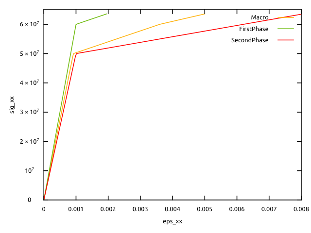
@Times {0.,1 in 50};The axial stress (uniform in the VER) is shown below as a function of the macroscopic axial strain, as a function of the axial strain of phase 1, and as a function of axial strain of phase 2.
We can see, as expected, that at a given stress value, the macroscopic strain is an average of local strains. When the macroscopic stress reaches the yield stress of one of the phases, the evolution of this phase becomes plastic, and this has repercussions on the macroscopic strain and on the other phase. The second phase becomes plastic later.