We present here an implementation of Taylor homogenization scheme [1] using BehaviourVariable keyword. This implementation allows using arbitrary local behaviours on each phase.

This tutorial first recalls the presentation of Taylor scheme, which is the generalization of Voigt scheme for non-linear behaviours. The derivation is very simple and allows to compute the tangent operator without resolving any non-linear problem. The local tangent operators are however needed.

Taylor homogenization scheme

Implementation in MFront

It is possible to implement this homogenization scheme through a Behaviour. This Behaviour must call the behaviour laws of each phase. So, an interesting solution is to use a BehaviourVariable.

Creation of the @BehaviourVariable

First step consists in creating variables which will allow to compute, on each phase, the local stress as a function of the local strain, and the local tangent operator as a function of the local strain. In short, it’s about being able to easily call a local Behaviour in the macroscopic Behaviour. These local Behaviour must be implemented before in .mfront files.

For the sake of simplicity, we will assume that we have 2 phases whose behaviour is elastoplastic with a Von Mises criterion with linear isotropic hardening. Material parameters are different between the phases. This behaviour is implemented in the file Plasticity.mfront, with the yield stress and hardening modulus as parameters.

@DSL IsotropicPlasticMisesFlow;
@Behaviour Plasticity;
@Epsilon 1e-14;
@UseQt true;

@MaterialProperty stress H;
@MaterialProperty stress s0;

@FlowRule {
  f = seq - H * p - s0;
  df_dseq = 1;
  df_dp = -H;
}

Then, in Taylor.mfront, we use the Default DSL:

@DSL Default;
@Behaviour Taylor;

Creation of BehaviourVariable is done as follows:

@BehaviourVariable b1 {
file: "Plasticity.mfront",
variables_suffix: "1",
external_names_prefix: "FirstPhase",
shared_external_state_variables: {".+"}
};

• the @BehaviourVariable block creates a variable named b1, representing our behaviour law on phase \(1\).
• the file implementing the behaviour law of phase \(1\) is specified by line \(2\).
• the variables of the behaviour law can be used with the name used by the implemented Behaviour, with an added suffix, here \(1\) for phase \(1\). For example, we can use eto1, the total strain of phase \(1\), or sig1 for the stress, and the same is true for other variables, e.g. eel1 or p1 for the cumulative plastic strain.
• the name of the variables outside, that is to say for example in the finite element code calling MFront, will have an added prefix FirstPhase, as specified by line \(4\).

For more details on using @BehaviourVariable, the reader can see the documentation of BehaviourVariable

Finally, it will be necessary to create 2 @BehaviourVariable for the 2 phases.

Implementation of Taylor scheme

After having defined the BehaviourVariable, we can implement the @Integrator block. Before this block, We specify that the tangent operator will be calculated inside the @Integrator block, given its very simple form, in the case of the Taylor scheme. This is done via @ProvidesTangentOperator.

@ProvidesTangentOperator;

@Integrator{
  b1.deto=deto;
  
  constexpr auto b1_smflag = TangentOperatorTraits<MechanicalBehaviourBase::STANDARDSTRAINBASEDBEHAVIOUR>::STANDARDTANGENTOPERATOR;
  const auto r1 = b1.integrate(b1_smflag,CONSISTENTTANGENTOPERATOR);
  StiffnessTensor Dt1 = b1.getTangentOperator();
 
  b2.deto=deto;
  
  constexpr auto b2_smflag = TangentOperatorTraits<MechanicalBehaviourBase::STANDARDSTRAINBASEDBEHAVIOUR>::STANDARDTANGENTOPERATOR;
  const auto r2 = b2.integrate(b2_smflag,CONSISTENTTANGENTOPERATOR);
  StiffnessTensor Dt2 = b2.getTangentOperator();
  
  updateAuxiliaryStateVariables(b1);
  updateAuxiliaryStateVariables(b2);

  sig = f * sig1 + (1 - f) * sig2;
  if (computeTangentOperator_) {
    Dt = f * Dt1 + (1 - f) * Dt2;
  }
}

We can see that we start by integrating the local behaviour. Let’s look on the first phase:

• line \(4\) specifies the strain increment on phase \(1\), in this case identical to the macroscopic strain increment deto. Furthermore, b1.eto is automatically initialized to eto1 before the integration of behaviour b1. This is automatic, and corresponds to call initialize(b1) before integration.
• the integration of behaviour b1 is done via line \(7\) with the integrate method which takes two arguments (see the documentation from @BehaviourVariable for more details). r1 is a boolean which is \(1\) if the integration went well.
• we retrieve the tangent operator via the getTangentOperator method.

Once local integrations have been carried out, it is necessary to update the auxiliary variables associated with each @BehaviourVariable. This is done on lines \(16\) and \(17\) with the updateAuxiliaryStateVariables function. This updates eto1 (resp. sig1) to the strain (resp. stress) obtained at the end of the integration of b1, and the same for the other variables like eel1 or p1. The same goes for b2.

Finally, the computation of macroscopic stress is given by Taylor scheme (average of local stresses) at line \(19\), and the macroscopic tangent operator is computed in the sequel.

Note that the following property had been defined before the @Integrator block:

@MaterialProperty real f;
f.setEntryName("FirstPhaseFraction");

Results

We then use MTest to simulate a uniaxial tensile test.

MTest file (Taylor.mtest) is the following:

@ModellingHypothesis 'Tridimensional';
@Behaviour<Generic> 'src/libBehaviour.so' 'Taylor';
@MaterialProperty<constant> 'FirstPhaseYoungModulus'     150.e9;
@MaterialProperty<constant> 'FirstPhasePoissonRatio'       0.35;
@MaterialProperty<constant> 'H1'                50.e9;
@MaterialProperty<constant> 's01'               200.e6;
@MaterialProperty<constant> 'SecondPhaseYoungModulus'     90.e9;
@MaterialProperty<constant> 'SecondPhasePoissonRatio'       0.3;
@MaterialProperty<constant> 'H2'                30.e9;
@MaterialProperty<constant> 's02'               50.e6;
@MaterialProperty<constant> 'FirstPhaseFraction' 0.1;
@ExternalStateVariable 'Temperature' 293.15;
@ImposedStrain 'EXX' {0 : 0, 1 : 3e-3};
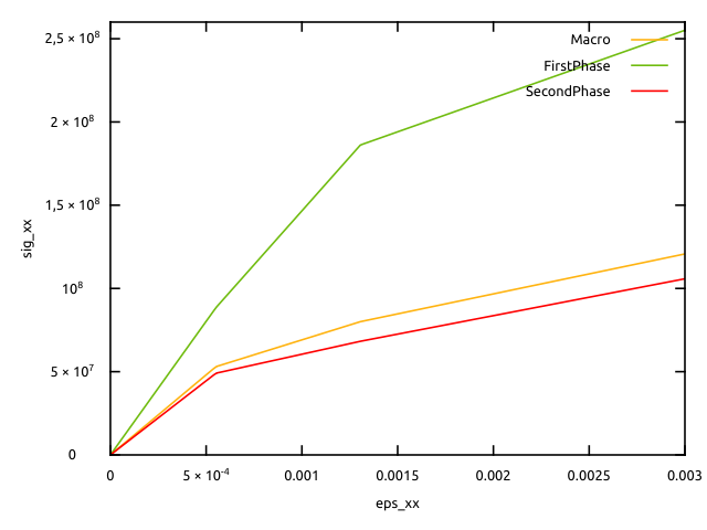
@Times {0, 1 in 200};

Macroscopic and local stresses are represented below as functions of the uniform axial strain:

We can see, as expected, that the macroscopic stress is an average of the local stresses. When the lowest yield stress is reached, the corresponding phase becomes plastic. The macroscopic tangent module is then reduced, which has repercussions on the macroscopic stress. The other phase becomes plastic later. Even if its evolution remains elastic, we can see that its axial stress is also impacted by the plastic transition of the other phase, because of the non-axial plastic strains appeared in this latter phase.