We present here an implementation of Ponte-Castaneda variational bound in non-linear elasticity [1]. It deals with the homogenization of a composite made of a matrix and spherical inclusions. The two phases have a non-linear elastic behaviour. The variational bound from Ponte-Castaneda is based on the computation of the strain second-moments.
This tutorial first recalls the scheme, and presents the implementation.
where \(N\) is the number of phases and \(\chi_r\) is characteristic function of phase \(r\).
The local potential \(w_r\) is a non-linear function of the strain \(\underline{\varepsilon}\), but here we focus on potentials of the form \[\begin{aligned} w_r(\underline{\varepsilon})={\displaystyle \frac{\displaystyle 9}{\displaystyle 2}} k_r\, \varepsilon_m^2+f_r (\varepsilon_{\mathrm{eq}}^2) \end{aligned}\] where \[\begin{aligned} \varepsilon_{\mathrm{eq}}= \sqrt{{\displaystyle \frac{\displaystyle 2}{\displaystyle 3}}\underline{\varepsilon}^d:\underline{\varepsilon}^d}\qquad\text{where}\quad \underline{\varepsilon}^d = \underline{\varepsilon}- {\displaystyle \frac{\displaystyle 1}{\displaystyle 3}} \mathrm{tr}\left(\underline{\varepsilon}\right)\underline{1} \qquad\text{and}\quad \varepsilon_m={\displaystyle \frac{\displaystyle 1}{\displaystyle 3}} \mathrm{tr}\left(\underline{\varepsilon}\right) \end{aligned}\] In the variational approach, the homogenization problem is equivalent to a minimization problem: \[\begin{aligned} \underline{\varepsilon}=\underset{\underline{\varepsilon}\in\mathcal K(\overline{\underline{\varepsilon}})}{\textrm{argmin}} \langle w(\underline{\varepsilon})\rangle \end{aligned}\]where the space of kinematically admissible fields \(\mathcal K(\overline{\underline{\varepsilon}})\) is introduced depending on the boundary conditions used, and it makes intervene the loading \(\overline{\underline{\varepsilon}}\) (which will be our total strain \(\texttt{eto}\)). The \(\langle.\rangle\) denotes the average on the representative volume element.
where \(c_r\) is the volume fraction of phase \(r\) and \(W_0^{\mathrm{eff}}(\overline{\underline{\varepsilon}})\) is the effective energy relative to a ‘linear comparison composite’ which is heterogeneous, and whose elastic moduli are the \(k_r\) and the \(\mu_0^r\).
The stationarity conditions associated to the minimization on \(\mu_0^r\) are: \[\begin{aligned} {\displaystyle \frac{\displaystyle \partial W_0^{\mathrm{eff}}}{\displaystyle \partial \mu_0^r}} = \dfrac{3c_r}{2}\,\left(f_r^*\right)'(\dfrac32 \mu_0^r) \end{aligned}\] which can be shown to be equivalent to \[\begin{aligned} \mu_0^r= {\displaystyle \frac{\displaystyle 2}{\displaystyle 3}} f_r'\left(\langle \varepsilon_{\mathrm{eq}}^2\rangle_r\right) \end{aligned}\] where \(\varepsilon_{\mathrm{eq}}\) is relative to \(\underline{\varepsilon}\) solution of the homogenization problem: \[\begin{aligned} \mathrm{div}\left(3k_r\,\varepsilon_m\,\underline{1}+2\mu_0^r\,\underline{\varepsilon}^d\right)=0,\qquad\underline{\varepsilon}\in\mathcal K(\overline{\underline{\varepsilon}}) \end{aligned}\] Besides, we can show (see [2], IX.B.) that the derivative of the effective energy of the linear composite w.r.t. the secant shear modulus gives the second-moment of the strain in this linear composite: \[\begin{aligned} \langle \varepsilon_{\mathrm{eq}}^2\rangle_r= {\displaystyle \frac{\displaystyle 2}{\displaystyle 3c_r}}{\displaystyle \frac{\displaystyle \partial W_0^{\mathrm{eff}}}{\displaystyle \partial \mu_0^r}} \end{aligned}\]where \(\underline{\mathbf{C}}_0^{\mathrm{eff}}\) is the effective elasticity of the linear comparison composite. In our case, we use Hashin-Shtrikman bounds.
The tangent operator is given by \[\begin{aligned} \dfrac{\mathrm{d}\overline{\underline{\sigma}}}{\mathrm{d}\overline{\underline{\varepsilon}}}=\underline{\mathbf{C}}_0^{\mathrm{eff}}+\dfrac{\mathrm{d}\underline{\mathbf{C}}_0^{\mathrm{eff}}}{\mathrm{d}\overline{\underline{\varepsilon}}} \end{aligned}\]Here, the derivative of \(\underline{\mathbf{C}}_0^{\mathrm{eff}}\) w.r.t. \(\overline{\underline{\varepsilon}}\) can be computed by derivating the Hashin-Shtrikman moduli w.r.t. the secant moduli \(\mu_0^r\) and the derivatives of these moduli w.r.t. \(\overline{\underline{\varepsilon}}\). However, it is tedious and in the implementation, we see that the convergence of the Newton Raphson algorithm is good if we only retain the first term \(\underline{\mathbf{C}}_0^{\mathrm{eff}}\) in the tangent operator.
The resolution hence consists in \[ \text{Find}\,e^r=\langle \varepsilon_{\mathrm{eq}}^2\rangle_r\,\text{such that}\quad\langle \varepsilon_{\mathrm{eq}}^2\rangle_r= {\displaystyle \frac{\displaystyle 2}{\displaystyle 3c_r}}{\displaystyle \frac{\displaystyle \partial W_0^{\mathrm{eff}}}{\displaystyle \partial \mu_0^r}} \] where \(W_0^{\mathrm{eff}}\) is the effective energy of a linear comparison composite whose elastic moduli are \(k_r\) annd \(\mu_0^r\) such that: \[ \mu_0^r= {\displaystyle \frac{\displaystyle 2}{\displaystyle 3}}{\displaystyle \frac{\displaystyle \partial f_r}{\displaystyle \partial e}}\left(\langle \varepsilon_{\mathrm{eq}}^2\rangle_r\right). \]
The iterative resolution of the non-linear equation can be summarized as \[ \underset{\substack{\\ \\ \\ \Downarrow\\ \\ \\\text{analytic / finite difference}\\ \\ \\\text{\texttt{@BehaviourVariable} / directly provided}}}{\mu_0^r= {\displaystyle \frac{\displaystyle 2}{\displaystyle 3}}{\displaystyle \frac{\displaystyle \partial f_r}{\displaystyle \partial e}}\left(\langle \varepsilon_{\mathrm{eq}}^2\rangle_r\right)}\quad\rightarrow\quad \underset{\substack{\\ \\ \\ \Downarrow\\ \\ \\\text{mean-field scheme / morphological tensors}\\ \\ \\\texttt{tfel::material::homogenization}}}{W_0^{\mathrm{eff}}\left(\mu_0^r\right)= \dfrac12\overline{\underline{\varepsilon}}:\underline{\mathbf{C}}_0^{\mathrm{eff}}:\overline{\underline{\varepsilon}}}\quad\rightarrow\quad\underset{\substack{\\ \\ \\ \Downarrow\\ \\ \\\text{analytic / finite difference}\\ \\ \\\texttt{tfel::material::homogenization}}}{\langle \varepsilon_{\mathrm{eq}}^2\rangle_r= {\displaystyle \frac{\displaystyle 2}{\displaystyle 3c_r}}{\displaystyle \frac{\displaystyle \partial W_0^{\mathrm{eff}}}{\displaystyle \partial \mu_0^r}}} \]
And the macroscopic stress must also be computed: \[ \overline{\underline{\sigma}}=\underline{\mathbf{C}}_0^{\mathrm{eff}}:\overline{\underline{\varepsilon}} \]
The first step of the resolution consists in computing the secant
modulus \(\mu_0^r\) and it can be done
analytically (as below) or via finite difference or automatic
differentiation. Moreover, for both strategies, we could use a
BehaviourVariable, defining the function \(f_r\) in an external file (in our example,
the function is to simple to do that).
The second step consists in computing the effective energy \(W_0^{\mathrm{eff}}\). This will be done via
tfel::material::homogenization. This namespace
provides classical mean-field schemes (we use a Hashin-Shtrikman bound
in our example below). This could also be done with interaction tensors,
providing externally. In another tutorial we show that we can
take into account more specifically the morphology of a polycrystal by
providing interaction tensors.
The third step consists in the computation of the second-moments.
This is also done via tfel::material::homogenization. Here
again, there are two strategies: analytical computation when possible,
and finite difference or automatic differentiation when the analytical
derivation is too tedious or even impossible. In our example below, the
computation is analytic.
where \(n\) is between \(0\) and \(1\), which means that \(f_r(e)=\dfrac{\sigma_r^0}{n+1}\,e^{\frac{n+1}2}\) (note that the function \(f_r\) is effectively concave relatively to \(e\), because \(0\lt n\leq 1\)).
Moreover, we make the choice of purely elastic inclusions. Hence, only the matrix is non-linear and has a secant modulus.
The unknowns of our non-linear problem are the \(e^r\). The secant moduli \(\mu_0^r\) can be computed by derivation of the function \(f_r\) which is given by the behaviour. In the precise case detailed above, we have \[\begin{aligned} {\displaystyle \frac{\displaystyle \partial f_r}{\displaystyle \partial e}}(e)=\dfrac{\sigma_r^0}{2}\,e^{\frac{n-1}2}\qquad\text{and}\quad\mu_0^r=\dfrac{\sigma_r^0}{3}\,\left(e^r\right)^{\frac{n-1}2} \end{aligned}\] Then, the effective energy of the linear comparison composite can be computed via a mean-field scheme. In our implementation, we proposed to use the Hashin-Shtrikman bound. The \(e^r\) must then cancel the following residue: \[\begin{aligned} r_{e^r}=e^r - {\displaystyle \frac{\displaystyle 2}{\displaystyle 3\,c_r}}{\displaystyle \frac{\displaystyle \partial W_0^{\mathrm{eff}}}{\displaystyle \partial \mu_0^r}} \end{aligned}\]which means that we only need the derivative of the Hashin-Shtrikman
bound. This will be given by the
tfel::material::homogenization functionalities.
The file PonteCastaneda1992.mfront is available in the
MFrontGallery project, here.
For the jacobian, we adopt the Numerical Jacobian, which
means that the beginning of the mfront file reads:
@DSL ImplicitII;
@Behaviour PC_VB_92;
@Author Martin Antoine;
@Date 12 / 12 / 25;
@Description{"Ponte Castaneda variational bounds for homogenization of non-linear elasticity (one potential), based on second-moments computation"};
@UseQt true;
@Algorithm NewtonRaphson_NumericalJacobian;
@PerturbationValueForNumericalJacobianComputation 1e-10;
@Epsilon 1e-12;
Moreover, the following libraries will be needed for computation of the stress and secant modulus:
@TFELLibraries {"Material"};
@Includes{
#include "TFEL/Material/IsotropicModuli.hxx"
#include "TFEL/Material/HomogenizationSecondMoments.hxx"
#include "TFEL/Material/LinearHomogenizationBounds.hxx"
}
We define two state variables which are the averages (on each phase) of the squares of the equivalent strains, and correspond to the \(e^r\):
@StateVariable real e_0;
e_0.setEntryName("MatrixSquaredEquivalentStrain");
@StateVariable real e_r;
e_r.setEntryName("InclusionSquaredEquivalentStrain");
The secant moduli are computed by derivation of function \(f_r\), which is detailed above. Hence
@Integrator {
//secant modulus/////////////////////////////////
const auto po = std::pow(max(e_0+de_0,real(1e-10)),0.5*(n_-1));
const auto mu0 = sig0/3.*po;
The second moment is given by the function
computeMeanSquaredEquivalentStrain (see documentation):
//second moments/////////////////////////////////
const auto em = tfel::math::trace(eto+deto)/3.;
const auto ed = tfel::math::deviator(eto+deto);
const auto em2 = em*em;
const auto eeq2 = 2./3.*(ed|ed);
using namespace tfel::material;
const auto kg0 = KGModuli<stress>(k_m,mu0);
const auto kgr = KGModuli<stress>(kar,mur);
using namespace tfel::material::homogenization::elasticity;
const auto eeq2_ = computeMeanSquaredEquivalentStrain(kg0,fr,kgr,em2,eeq2);
const auto eeq20=std::get<0>(eeq2_);
const auto eeq2r=std::get<1>(eeq2_);
Now we can write the residues:
There is no jacobian because we use the
NumericalJacobian. The macroscopic stress is given by the
Hashin-Shtrikman lower bound (indeed, the lower bound is better suited
for soft matrix and rigid inclusions):
//sigma//////////////////////////////////////
vector<real> tab_f={1-fr,fr};
vector<stress> tab_k = {k_m,kar};
vector<stress> tab_mu = {mu0,mur};
const auto HSB=computeIsotropicHashinShtrikmanBounds<3,stress>(tab_f,tab_k,tab_mu);
const auto LB=std::get<0>(HSB);
const auto kHS=std::get<0>(LB);
const auto muHS=std::get<1>(LB);
Chom=3*kHS*J+2*muHS*K;
sig = Chom*(eto+deto);
}
(Note that Chom is the effective elastic tensor, defined
here as a local variable). Afterwards, we can give the tangent
operator:
We then use MTest to simulate a strain-imposed test.
MTest file is the following:
@ModellingHypothesis 'Tridimensional';
@Behaviour<Generic> 'src/libBehaviour.so' 'PC_VB_92';
@ExternalStateVariable 'Temperature' {0 : 1000,1:1000};
@MaterialProperty<constant> 'sig0' 1.e9;
@MaterialProperty<constant> 'n_' 0.05;
@MaterialProperty<constant> 'k_m' 1.e9;
@MaterialProperty<constant> 'kar' 1.e15;
@MaterialProperty<constant> 'mur' 1.e15;
@MaterialProperty<constant> 'fr' 0.25;
@ImposedStrain 'EXX' {0 : 0, 100 : 0.8660254};
@ImposedStrain 'EYY' {0 : 0, 100 : -0.8660254};
@ImposedStrain 'EZZ' {0 : 0, 100 : 0};
@ImposedStrain 'EXY' {0 : 0, 100 : 0};
@ImposedStrain 'EXZ' {0 : 0, 100 : 0};
@ImposedStrain 'EYZ' {0 : 0, 100 : 0};
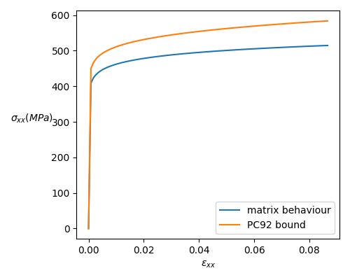
@Times {0.,10 in 100};The macroscopic stress \(\sigma_{xx}\) is represented below as a function of the macroscopic strain \(\varepsilon_{xx}\):
We also plotted the behaviour of the matrix when there is no inclusions (it gives an idea of the reinforcement given by the inclusions).