This tutorial explains how to implement Cailletaud-Pilvin \(\beta\)-rule [1] in the context of elasto-viscoplastic composites using an arbitrary local flow function. In this tutorial, a local behaviour of Meric-Cailletaud type [2] is proposed.
Here, the implementation of this homogenization scheme requires the
local tangent operators, obtained via the integration of a local
Behaviour.
We first recall Cailletaud-Pilvin \(\beta\)-rule and present the non-linear
system derived from it. We then implement it in MFront and
explain how to use the keyword @BehaviourVariable for the
integration of the local behaviours.
where \(f_i\) is a non-linear function.
Assuming that \(\phi_i\) is volume fraction of phase \(i\), the macroscopic strain field is defined as \[\begin{aligned} \underline{E}= \sum_i \phi_i \underline{\epsilon}^{\mathrm{to}}_i \\ \end{aligned}\]and is given as a parameter.
In this context, the proposition is to introduce an internal variable \(\underline{\beta}_i\) on each phase, whose evolution is given by \[\begin{aligned} \underline{\dot{\beta}}_i= \underline{\dot{\epsilon}}^{\mathrm{vp}}_i-D\,||\underline{\dot{\epsilon}}^{\mathrm{vp}}_i||\,\underline{\beta}_i \\ \end{aligned}\] where \(D\in\mathbb R\) is a parameter and \[\begin{aligned} ||\underline{\dot{\epsilon}}^{\mathrm{vp}}_i||=\sqrt{\dfrac 23 \underline{\dot{\epsilon}}^{\mathrm{vp}}_i\mathbin{\mathord{:}}\underline{\dot{\epsilon}}^{\mathrm{vp}}_i}. \\ \end{aligned}\] The localisation relation is also proposed: \[\begin{aligned} \underline{\sigma}_i= \underline{\Sigma}+ c\,(\underline{B}-\underline{\beta}_i) \\ \end{aligned}\] where \(c\) is a real parameter, \(\underline{B}\) is a macroscopic variable: \[\begin{aligned} \underline{B}= \sum_i \phi_i\underline{\beta}_i\\ \end{aligned}\] and \(\underline{\Sigma}\) is the macroscopic stress, which verifies (by averaging the localisation relation) \[\begin{aligned} \underline{\Sigma}= \sum_i \phi_i\underline{\sigma}_i\\ \end{aligned}\]We discretize the time interval and look for the increment of the variables. We choose \(\Delta\underline{\epsilon}^{\mathrm{to}}_i\), \(\Delta{\underline{\beta}}_i\) and \(\Delta{\underline{\sigma}}\) as unknowns of our non-linear system:
\(\left\{ \begin{aligned} &\sum_{i=1}^{N}\phi_i\,\Delta\underline{\epsilon}^{\mathrm{to}}_i - \Delta\underline{E} = 0\\ &\Delta{\underline{\sigma}}_i\left(\underline{\epsilon}^{\mathrm{to}}_i,\Delta\underline{\epsilon}^{\mathrm{to}}_i\right)-\Delta{\underline{\sigma}}- c\,(\Delta\underline{B}-\Delta\underline{\beta}_i) = 0\qquad\forall i\\ &\Delta\underline{\beta}_i - \Delta\underline{\epsilon}^{\mathrm{vp}}_i\left(\underline{\epsilon}^{\mathrm{to}}_i,\Delta\underline{\epsilon}^{\mathrm{to}}_i\right)+ D\,||\Delta\underline{\epsilon}^{\mathrm{vp}}_i\left(\underline{\epsilon}^{\mathrm{to}}_i,\Delta\underline{\epsilon}^{\mathrm{to}}_i\right)||\,(\underline{\beta}_i+\theta\Delta\underline{\beta}_i)=0\qquad\forall i\\ \end{aligned}\right.\)
where the following auxiliary variable is introduced:
\(\begin{aligned} &\Delta\underline{B} = \sum_{i=1}^{N}\phi_i\,\Delta\underline{\beta}_i\\ \end{aligned}\) and where \(\Delta{\underline{\sigma}}_i\left(\underline{\epsilon}^{\mathrm{to}}_i,\Delta\underline{\epsilon}^{\mathrm{to}}_i\right)\) and \(\Delta\underline{\epsilon}^{\mathrm{vp}}_i\left(\underline{\epsilon}^{\mathrm{to}}_i,\Delta\underline{\epsilon}^{\mathrm{to}}_i\right)\) are obtained with the integration of the local behaviours. Indeed, we have \(\Delta\underline{\epsilon}^{\mathrm{vp}}_i\left(\underline{\epsilon}^{\mathrm{to}}_i,\Delta\underline{\epsilon}^{\mathrm{to}}_i\right)=\Delta\underline{\epsilon}^{\mathrm{to}}_i-\underline{S}_i\mathbin{\mathord{:}}\Delta{\underline{\sigma}}_i\left(\underline{\epsilon}^{\mathrm{to}}_i,\Delta\underline{\epsilon}^{\mathrm{to}}_i\right)\). Note that the local elastic strain can also be computed with this local integration.
To solve this non-linear problem in MFront, we use the
ImplicitII DSL (because we do not consider
\(\underline{\epsilon}^{\mathrm{el}}\)
as an integration variable). We only have to precise the residues and
the Jacobian matrix. The residues are:
\(\left\{ \begin{aligned} &f_{\underline{E}}=\sum_{i=1}^{N}\phi_i\,\Delta\underline{\epsilon}^{\mathrm{to}}_i - \Delta\underline{E}\\ &f_{\underline{\epsilon}^{\mathrm{to}}_i} =\frac{1}{\sigma_0}\left[\Delta{\underline{\sigma}}_i\left(\underline{\epsilon}^{\mathrm{to}}_i,\Delta\underline{\epsilon}^{\mathrm{to}}_i\right)-\Delta{\underline{\sigma}}- c\,(\Delta\underline{B}-\Delta\underline{\beta}_i)\right] \qquad \forall i\\ &f_{\underline{\beta}_i} =\Delta\underline{\beta}_i - \Delta\underline{\epsilon}^{\mathrm{vp}}_i\left(\underline{\epsilon}^{\mathrm{to}}_i,\Delta\underline{\epsilon}^{\mathrm{to}}_i\right)+D\,||\Delta\underline{\epsilon}^{\mathrm{vp}}_i\left(\underline{\epsilon}^{\mathrm{to}}_i,\Delta\underline{\epsilon}^{\mathrm{to}}_i\right)||\,(\underline{\beta}_i+\theta\Delta\underline{\beta}_i) \qquad \forall i\\ \end{aligned}\right.\)
where \(\sigma_{0}\) is a parameter that gives the same dimension and magnitude to the residues. The jacobian matrix is given by
\(\left\{ \begin{aligned} &{\displaystyle \frac{\displaystyle \partial f_{\underline{E}}}{\displaystyle \partial \Delta{\underline{\sigma}}}} = \underline{\mathbf{0}}\\ &{\displaystyle \frac{\displaystyle \partial f_{\underline{E}}}{\displaystyle \partial \Delta\underline{\epsilon}^{\mathrm{to}}_j}} = \phi_j\underline{\mathbf{I}}\qquad \forall j\\ &{\displaystyle \frac{\displaystyle \partial f_{\underline{E}}}{\displaystyle \partial \Delta{\underline{\beta}}_j}} = \underline{\mathbf{0}}\qquad \forall j\\ &{\displaystyle \frac{\displaystyle \partial f_{\underline{\epsilon}^{\mathrm{to}}_i}}{\displaystyle \partial \Delta{\underline{\sigma}}}} = -\frac{1}{\sigma_0}\underline{\mathbf{I}}\qquad \forall i\\ &{\displaystyle \frac{\displaystyle \partial f_{\underline{\epsilon}^{\mathrm{to}}_i}}{\displaystyle \partial \Delta\underline{\epsilon}^{\mathrm{to}}_j}} = \frac{\delta_{ij}}{\sigma_0}\,{\displaystyle \frac{\displaystyle \partial \underline{\sigma}_j}{\displaystyle \partial \underline{\epsilon}^{\mathrm{to}}_j}}\left(\underline{\epsilon}^{\mathrm{to}}_j,\Delta\underline{\epsilon}^{\mathrm{to}}_j\right)\qquad\forall i,j\\ &{\displaystyle \frac{\displaystyle \partial f_{\underline{\epsilon}^{\mathrm{to}}_i}}{\displaystyle \partial \Delta{\underline{\beta}}_j}} = \frac{c}{\sigma_0}\,(\delta_{ij}-\phi_j)\underline{\mathbf{I}}\qquad \forall i,j\\ &{\displaystyle \frac{\displaystyle \partial f_{\underline{\beta}_i}}{\displaystyle \partial \Delta{\underline{\sigma}}}} = \underline{\mathbf{0}}\qquad \forall i\\ &{\displaystyle \frac{\displaystyle \partial f_{\underline{\beta}_i}}{\displaystyle \partial \Delta\underline{\epsilon}^{\mathrm{to}}_j}} = -\delta_{ij}\,{\displaystyle \frac{\displaystyle \partial \underline{\sigma}_j}{\displaystyle \partial \underline{\epsilon}^{\mathrm{to}}_j}}\left(\underline{\epsilon}^{\mathrm{to}}_j,\Delta\underline{\epsilon}^{\mathrm{to}}_j\right)+D\,(\underline{\beta}_i+\theta\Delta\underline{\beta}_i)\otimes{\displaystyle \frac{\displaystyle \partial ||\Delta\underline{\epsilon}^{\mathrm{vp}}_i||}{\displaystyle \partial \Delta\underline{\epsilon}^{\mathrm{to}}_j}}\qquad \forall i,j\\ &{\displaystyle \frac{\displaystyle \partial f_{\underline{\beta}_i}}{\displaystyle \partial \Delta{\underline{\beta}}_j}} = \left(1+\theta\,D\,||\Delta\underline{\epsilon}^{\mathrm{vp}}_i||\right)\,\delta_{ij}\,\underline{\mathbf{I}} \qquad \forall i,j\\ \end{aligned}\right.\)
where \(||\Delta\underline{\epsilon}^{\mathrm{vp}}_i||\) is used for \(||\Delta\underline{\epsilon}^{\mathrm{vp}}_i\left(\underline{\epsilon}^{\mathrm{to}}_i,\Delta\underline{\epsilon}^{\mathrm{to}}_i\right)||\). Moreover,
\(\left\{ \begin{aligned} {\displaystyle \frac{\displaystyle \partial ||\Delta\underline{\epsilon}^{\mathrm{vp}}_i||}{\displaystyle \partial \Delta\underline{\epsilon}^{\mathrm{to}}_j}}&=\frac 23\delta_{ij}{\displaystyle \frac{\displaystyle \Delta\underline{\epsilon}^{\mathrm{vp}}_i}{\displaystyle ||\Delta\underline{\epsilon}^{\mathrm{vp}}_i||}}\mathbin{\mathord{:}}{\displaystyle \frac{\displaystyle \partial \Delta\underline{\epsilon}^{\mathrm{vp}}_i}{\displaystyle \partial \Delta\underline{\epsilon}^{\mathrm{to}}_j}}\left(\underline{\epsilon}^{\mathrm{to}}_i,\Delta\underline{\epsilon}^{\mathrm{to}}_i\right)\\ &=\frac 23\delta_{ij}{\displaystyle \frac{\displaystyle \Delta\underline{\epsilon}^{\mathrm{vp}}_i}{\displaystyle ||\Delta\underline{\epsilon}^{\mathrm{vp}}_i||}}\mathbin{\mathord{:}}\left({\displaystyle \frac{\displaystyle \partial \Delta\underline{\epsilon}^{\mathrm{to}}_i}{\displaystyle \partial \Delta\underline{\epsilon}^{\mathrm{to}}_j}}-{\displaystyle \frac{\displaystyle \partial \Delta\underline{\epsilon}^{\mathrm{el}}_i}{\displaystyle \partial \Delta\underline{\epsilon}^{\mathrm{to}}_j}}\right)\\ &=\frac 23\delta_{ij}{\displaystyle \frac{\displaystyle \Delta\underline{\epsilon}^{\mathrm{vp}}_i}{\displaystyle ||\Delta\underline{\epsilon}^{\mathrm{vp}}_i||}}\mathbin{\mathord{:}}\left(\delta_{ij}\underline{\mathbf{I}}-\delta_{ij}\underline{\mathbf{S}}_j\mathbin{\mathord{:}}{\displaystyle \frac{\displaystyle \partial \Delta{\underline{\sigma}}_j}{\displaystyle \partial \Delta\underline{\epsilon}^{\mathrm{to}}_j}}\right)\\ \end{aligned}\right.\)
We can see the term \({\displaystyle \frac{\displaystyle \partial \Delta{\underline{\sigma}}_j}{\displaystyle \partial \Delta\underline{\epsilon}^{\mathrm{to}}_j}}\), that will be provided by the local integration.
Hence, the following equality is still verified:
\[\begin{aligned} {\displaystyle \frac{\displaystyle \partial \Delta Y}{\displaystyle \partial \Delta\underline{E}}}&=-\mathbf{J}^{-1}\cdot{\displaystyle \frac{\displaystyle \partial F}{\displaystyle \partial \Delta \underline{E}}}\\ \end{aligned}\]where \(\mathbf{J}={\displaystyle \frac{\displaystyle \partial F}{\displaystyle \partial \Delta Y}}\) is the Jacobian of the system.
Given the form of \({\displaystyle \frac{\displaystyle \partial F}{\displaystyle \partial \Delta \underline{E}}}\), \({\displaystyle \frac{\displaystyle \partial \Delta{\underline{\sigma}}}{\displaystyle \partial \Delta\underline{E}}}\) can be retrieved from the \(6\times 6\) upper-left submatrix of \(\mathbf{J}^{-1}\).
The implementation requires the integration of the local behaviours.
These are carried out via the @BehaviourVariable keyword.
The implementation of the local behaviour is explained here.
All files
MericCailletaudSingleCrystalViscoPlasticity.mfront,
BetaRule.mfront and BetaRule.mtest are
available in the MFrontGallery project, here.
For the example, we assume that the composite is made of only 2 phases. We hence define the integration variables:
@StateVariable Stensor Sig;
Sig.setEntryName("MacroscopicStress");
@StateVariable Stensor eto1;
eto1.setEntryName("FirstPhaseTotalStrain");
@StateVariable Stensor eto2;
eto2.setEntryName("SecondPhaseTotalStrain");
@StateVariable Stensor beta1;
beta1.setEntryName("FirstPhaseBetaStrain");
@StateVariable Stensor beta2;
beta2.setEntryName("SecondPhaseBetaStrain");
and we define the local behaviours with
@BehaviourVariable:
@BehaviourVariable b1 {
file: "MericCailletaudSingleCrystalViscoPlasticity.mfront",
variables_suffix: "1",
store_gradients: false,
external_names_prefix: "FirstPhase",
shared_external_state_variables: {".+"}
};
(the same for phase 2).
We note that the gradients are not stored because the
StateVariable eto1 (resp. eto2)
are defined.
The integration of the local behaviour is performed as follows:
  initialize(b1);
  b1.eto=eto1;
  b1.deto=deto1;
  constexpr auto b1_smflag = TangentOperatorTraits<MechanicalBehaviourBase::STANDARDSTRAINBASEDBEHAVIOUR>::STANDARDTANGENTOPERATOR;
  const auto r1 = b1.integrate(b1_smflag,CONSISTENTTANGENTOPERATOR);
  StiffnessTensor Dt1 = b1.getTangentOperator();
and the following variables are stored:
  auto dsig1=b1.sig-sig1;
  auto deel1=b1.eel-eel1;
  auto devp1=deto1-deel1;
  auto ndevp_1=sqrt(real(2)/3*devp1|devp1);
  auto beta_mts_1=beta1+theta*dbeta1;
The same goes for phase 2. Here are the residues:
  //residues
  auto dB=(1-f)*dbeta1+f*dbeta2;
  fSig = -deto+ (1-f)*deto1+f*deto2;
  feto1 = (dsig1-dSig-c*(dB-dbeta1))/sig_0;
  feto2 = (dsig2-dSig-c*(dB-dbeta2))/sig_0;
  fbeta1 = dbeta1-devp1+DD*ndevp_1*beta_mts_1;
  fbeta2 = dbeta2-devp2+DD*ndevp_2*beta_mts_2;
and the terms of the analytical jacobian:
  //jacobian matrix
  auto Null = Stensor4{real{}};
  dfSig_ddSig=Null;
  dfSig_ddeto1 = (1-f)*Id;
  dfSig_ddeto2 = f*Id;

  dfeto1_ddSig = -Id/sig_0;
  dfeto2_ddSig = -Id/sig_0;

  dfeto1_ddeto1 = Dt1/sig_0;
  dfeto2_ddeto2 = Dt2/sig_0;

  dfeto1_ddbeta1 = c/sig_0*f*Id;
  dfeto1_ddbeta2 = -c/sig_0*f*Id;
  dfeto2_ddbeta1 = c/sig_0*(f-1)*Id;
  dfeto2_ddbeta2 = c/sig_0*(1-f)*Id;

  dfbeta1_ddeto1 = -(Id-S1*Dt1) + 2*DD/3*Stensor4(beta_mts_1^devp1)*Stensor4(Id-S1*Dt1)/max(ndevp_1,eeps);
  dfbeta2_ddeto2 = -(Id-S2*Dt2) + 2*DD/3*Stensor4(beta_mts_2^devp2)*Stensor4(Id-S2*Dt2)/max(ndevp_2,eeps);

  dfbeta1_ddbeta1 =Id+ theta*DD*ndevp_1*Id;
  dfbeta2_ddbeta2 =Id+ theta*DD*ndevp_2*Id;
Note that S1 and S2 are the compliance
tensors of each phase and were defined by the elastic coefficients of
each phase. The computation of the stress and of the tangent operator is
straightforward:
@ComputeFinalStress{
  sig += dSig;
}

@TangentOperator{
  Stensor4 iJs;
  getPartialJacobianInvert(iJs);
  Dt=iJs;
}
Note that getPartialJacobianInvert(iJs) allows obtaining
the 6x6 left-upper part of the inverse of the Jacobian. The left-upper
part is associated with the first integration variable declared (here
Sig).
We used MTest to carry out simulations of a uniaxial
tensile test on a two-grain polycrystal. The first phase is stiffer than
the second, and we also choose for the example a different Norton
exponent between the phases. The following values are given by the
mtest file:
@ModellingHypothesis 'Tridimensional';
@Behaviour<Generic> 'src/libBehaviour.so' 'BetaRuleBehaviour';
@MaterialProperty<constant> 'FirstPhaseFraction' 0.5;
@MaterialProperty<constant> 'E_1' 208000;
@MaterialProperty<constant> 'nu_1' 0.3;
@MaterialProperty<constant> 'mu_1' 80000;
@MaterialProperty<constant> 'E_2' 104000;
@MaterialProperty<constant> 'nu_2' 0.3;
@MaterialProperty<constant> 'mu_2' 40000;
@MaterialProperty<constant> 'tau01' 36.;
@MaterialProperty<constant> 'tau02' 25.;
@MaterialProperty<constant> 'n1' 10.;
@MaterialProperty<constant> 'n2' 5.;
@ExternalStateVariable 'Temperature' 293.15;
@ImposedStrain 'EXX' {0 : 0, 5 :1e-2};
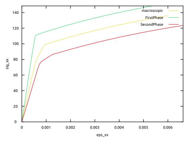
@Times {0, 3 in 400};Note that the elastic behaviours are isotropic for the example. (the file is available in the archive). We plotted here the macroscopic and local behaviours (\(\underline{\sigma}_i\) as a function of \(\underline{\epsilon}_i\)).
When a huge number of phases are involved in the microstructure, the non-linear system previously presented becomes huge and the static condensation allows handling this high number of unknowns. Indeed, the linear system resolved at each step of the Newton algorithm is reduced by using only the macroscopic variables \(\Delta\underline{B}\) and \(\Delta\underline{\Sigma}\) as unknowns in this system. The increments of the local unknowns are deduced afterwards.
Here we want to reduce our system and choose \(\Delta\underline{B}\), \(\Delta\underline{\Sigma}\) as the main unknowns.
To that extent, we first express the Newton-Raphson increments \(\delta\Delta\underline{\epsilon}^{\mathrm{to}}_i\) and \(\delta\Delta\underline{\beta}_i\) as functions of the increments \(\delta\Delta\underline{B}\) and \(\delta\Delta\underline{\Sigma}\). We have
\(-\underline{r}_{\underline{\epsilon}_i}=\dfrac{\partial \underline{r}_{\underline{\epsilon}_i}}{\partial \Delta\underline{B}}\mathbin{\mathord{:}}\delta\Delta\underline{B}+\dfrac{\partial \underline{r}_{\underline{\epsilon}_i}}{\partial \Delta\underline{\Sigma}}\mathbin{\mathord{:}}\delta\Delta\underline{\Sigma}+\dfrac{\partial \underline{r}_{\underline{\epsilon}_i}}{\partial \Delta\underline{\beta}_i}\mathbin{\mathord{:}}\delta\Delta\underline{\beta}_i+\dfrac{\partial \underline{r}_{\underline{\epsilon}_i}}{\partial \Delta\underline{\epsilon}_i}\mathbin{\mathord{:}}\delta\Delta\underline{\epsilon}^{\mathrm{to}}_i\)
with
\[\begin{aligned} &\dfrac{\partial \underline{r}_{\underline{\epsilon}_i}}{\partial \Delta\underline{B}}=-\frac{c}{\sigma_0}\,\underline{\mathbf{I}}, \qquad\qquad \dfrac{\partial \underline{r}_{\underline{\epsilon}_i}}{\partial \Delta\underline{\Sigma}}=-\frac{1}{\sigma_0}\,\underline{\mathbf{I}} \\ &\dfrac{\partial \underline{r}_{\underline{\epsilon}_i}}{\partial \Delta\underline{\beta}_i} =\frac{c}{\sigma_0}\,\underline{\mathbf{I}},\qquad\qquad \dfrac{\partial \underline{r}_{\underline{\epsilon}_i}}{\partial \Delta\underline{\epsilon}^{\mathrm{to}}_i} =\frac{1}{\sigma_0}\,\dfrac{\partial\Delta{\underline{\sigma}}_i}{\partial\Delta\underline{\epsilon}^{\mathrm{to}}_i} \\ \end{aligned}\]Let us now do the same with the second residue:
\(-\underline{r}_{\underline{\beta}_i}=\dfrac{\partial \underline{r}_{\underline{\beta}_i}}{\partial \Delta\underline{\beta}_i}\mathbin{\mathord{:}}\delta\Delta\underline{\beta}_i+\dfrac{\partial \underline{r}_{\underline{\beta}_i}}{\partial \Delta\underline{\epsilon}^{\mathrm{to}}_i}\mathbin{\mathord{:}}\delta\Delta\underline{\epsilon}^{\mathrm{to}}_i\)
with \[\begin{aligned} &\dfrac{\partial \underline{r}_{\underline{\beta}_i}}{\partial \Delta\underline{\beta}_i} =\left(1+\theta\,D\,||\Delta\underline{\epsilon}^{\mathrm{vp}}_i||\right)\underline{\mathbf{I}}\\ &\dfrac{\partial \underline{r}_{\underline{\beta}_i}}{\partial \Delta\underline{\epsilon}^{\mathrm{to}}_i} = \left(\frac {2D}3\,{\underline{\beta}_i|}_{t+\theta\Delta t}\otimes\underline{n}_i-\underline{\mathbf{I}}\right)\mathbin{\mathord{:}}\dfrac{\partial\underline{\epsilon}^{\mathrm{vp}}_i}{\partial\Delta\underline{\epsilon}^{\mathrm{to}}_i},\qquad\underline{n}_i&=\dfrac{\Delta\underline{\epsilon}^{\mathrm{vp}}_i}{||\Delta\underline{\epsilon}^{\mathrm{vp}}_i||}\\ \end{aligned}\]and \(\underline{\mathbf{I}}\) is the fourth-rank identity tensor.
Due to its form, \(\dfrac{\partial \underline{r}_{\underline{\beta}_i}}{\partial \Delta\underline{\beta}_i}\) is invertible. Hence,
\(\delta\Delta\underline{\beta}_i=-\left(\dfrac{\partial \underline{r}_{\underline{\beta}_i}}{\partial \Delta\underline{\beta}_i}\right)^{-1}\mathbin{\mathord{:}}\left[\underline{r}_{\underline{\beta}_i}+\dfrac{\partial \underline{r}_{\underline{\beta}_i}}{\partial \Delta\underline{\epsilon}^{\mathrm{to}}_i}\mathbin{\mathord{:}}\delta\Delta\underline{\epsilon}^{\mathrm{to}}_i\right]\)
and this can be put into the residue \(r_{\underline{\epsilon}_i}\):
\(-\underline{r}_{\underline{\epsilon}_i}-\dfrac{\partial \underline{r}_{\underline{\epsilon}_i}}{\partial \Delta\underline{B}}\mathbin{\mathord{:}}\delta\Delta\underline{B}-\dfrac{\partial \underline{r}_{\underline{\epsilon}_i}}{\partial \Delta\underline{\Sigma}}\mathbin{\mathord{:}}\delta\Delta\underline{\Sigma}=\underline{\mathbf{a}}_i\mathbin{\mathord{:}}\delta\Delta\underline{\varepsilon}_i+\underline{b}_i\)
with \(\underline{\mathbf{a}}_i=-\dfrac{\partial \underline{r}_{\underline{\epsilon}_i}}{\partial \Delta\underline{\beta}_i}\mathbin{\mathord{:}}\left(\dfrac{\partial \underline{r}_{\underline{\beta}_i}}{\partial \Delta\underline{\beta}_i}\right)^{-1}\mathbin{\mathord{:}}\dfrac{\partial \underline{r}_{\underline{\beta}_i}}{\partial \Delta\underline{\epsilon}_i}+\dfrac{\partial \underline{r}_{\underline{\epsilon}_i}}{\partial \Delta\underline{\epsilon}_i},\qquad \underline{b}_i = -\dfrac{\partial \underline{r}_{\underline{\epsilon}_i}}{\partial \Delta\underline{\beta}_i}\mathbin{\mathord{:}}\left(\dfrac{\partial \underline{r}_{\underline{\beta}_i}}{\partial \Delta\underline{\beta}_i}\right)^{-1}\mathbin{\mathord{:}}\underline{r}_{\underline{\beta}_i}\)
Here, if \(\underline{\mathbf{a}}_i\) is not invertible, this means that the Newton-Raphson algorithm will fail to solve the non-linear system, which is independent of the static condensation. Hence, we assume \(\underline{a}_i\) is invertible and we write
\(\delta\Delta\underline{\epsilon}^{\mathrm{to}}_i=\underline{\mathbf{a}}_i^{-1}\mathbin{\mathord{:}}\left[-\underline{r}_{\underline{\epsilon}_i}-\dfrac{\partial \underline{r}_{\underline{\epsilon}_i}}{\partial \Delta\underline{B}}\mathbin{\mathord{:}}\delta\Delta\underline{B}-\dfrac{\partial \underline{r}_{\underline{\epsilon}_i}}{\partial \Delta\underline{\Sigma}}\mathbin{\mathord{:}}\delta\Delta\underline{\Sigma}-\underline{b}_i\right]\)
\(\delta\Delta\underline{\epsilon}^{\mathrm{to}}_i,\delta\Delta\underline{\beta}_i\) can then be expressed as functions of \(\delta\Delta\underline{B}\), \(\delta\Delta\underline{\Sigma}\) via the ‘decondensation relations’.
Coming back to the residue \(\underline{r}_{\underline{E}}\) and \(\underline{r}_{\underline{B}}\):
\[\begin{aligned} -\underline{r}_{\underline{E}}&=\sum_i f_i \delta\Delta\underline{\epsilon}^{\mathrm{to}}_i\\ -\underline{r}_{\underline{B}}&=\delta\Delta\underline{B}-\sum_i f_i \delta\Delta\underline{\beta}_i\\ \end{aligned}\]and replacing \(\delta\Delta\underline{\epsilon}^{\mathrm{to}}_i\) and \(\delta\Delta\underline{\beta}_i\) by their expressions,
\[\begin{equation} \begin{pmatrix} \underline{\mathbf{P}}&\underline{\mathbf{Q}}\\ \underline{\mathbf{R}}&\underline{\mathbf{S}}\\ \end{pmatrix} \cdot \begin{pmatrix} \delta\Delta\underline{\Sigma}\\ \delta\Delta\underline{B} \end{pmatrix} = \begin{pmatrix} -\underline{r}_{\underline{E}}-\underline{T}\\ -\underline{r}_{\underline{B}}-\underline{U} \end{pmatrix} \end{equation}\] where
\[\begin{aligned} \underline{\mathbf{P}}&=-\sum_i f_i\underline{\mathbf{a}}_i^{-1}\mathbin{\mathord{:}}\dfrac{\partial \underline{r}_{\underline{\epsilon}_i}}{\partial \Delta\underline{\Sigma}},\qquad\underline{\mathbf{Q}}=-\sum_i f_i\underline{\mathbf{a}}_i^{-1}\mathbin{\mathord{:}}\dfrac{\partial \underline{r}_{\underline{\epsilon}_i}}{\partial \Delta\underline{B}}\\ \underline{\mathbf{R}}&=-\sum_i f_i \left(\dfrac{\partial \underline{r}_{\underline{\beta}_i}}{\partial \Delta\underline{\beta}_i}\right)^{-1}\mathbin{\mathord{:}}\dfrac{\partial \underline{r}_{\underline{\beta}_i}}{\partial \Delta\underline{\epsilon}_i}\mathbin{\mathord{:}}\underline{\mathbf{a}}_i^{-1}\mathbin{\mathord{:}}\dfrac{\partial \underline{r}_{\underline{\epsilon}_i}}{\partial \Delta\underline{\Sigma}}\\ \underline{\mathbf{S}}&=\underline{I}-\sum_i f_i\left(\dfrac{\partial \underline{r}_{\underline{\beta}_i}}{\partial \Delta\underline{\beta}_i}\right)^{-1}\mathbin{\mathord{:}}\dfrac{\partial \underline{r}_{\underline{\beta}_i}}{\partial \Delta\underline{\epsilon}_i}\mathbin{\mathord{:}}\underline{\mathbf{a}}_i^{-1}\mathbin{\mathord{:}}\dfrac{\partial \underline{r}_{\underline{\epsilon}_i}}{\partial \Delta\underline{B}}\\ \underline{T}&=-\sum_i f_i\underline{\mathbf{a}}_i^{-1}\mathbin{\mathord{:}}\left(\underline{r}_{\underline{\varepsilon}_i}+\underline{b}_i\right),\qquad\underline{U}=\sum_i f_i \left(\dfrac{\partial \underline{r}_{\underline{\beta}_i}}{\partial \Delta\underline{\beta}_i}\right)^{-1}\mathbin{\mathord{:}}\left[\underline{r}_{\underline{\beta}_i}-\dfrac{\partial \underline{r}_{\underline{\beta}_i}}{\partial \Delta\underline{\epsilon}_i}\mathbin{\mathord{:}}\underline{\mathbf{a}}_i^{-1}\mathbin{\mathord{:}}\left(\underline{r}_{\underline{\varepsilon}_i}+\underline{b}_i\right)\right]\\ \end{aligned}\]We can see that \(\delta\Delta\underline{\Sigma}\) and \(\delta\Delta\underline{B}\) are solutions of a \(12\times 12\) linear system, whose matrix is the jacobian matrix, noted \(\underline{J}\) in the following. Here again, the existence of a unique solution to this system is strongly correlated to the convergence of the global Newton-Raphson algorithm, convergence which is independent of the static condensation.
The computation of the tangent operator is similar to above. Indeed, we can define \(\Delta \underline{Y}=(\Delta \underline{\Sigma},\Delta \underline{B})\), and \(\underline{R}=(\underline{r}_{\underline{E}},\underline{r}_{\underline{B}})\) so that for every \(\Delta\underline{E}\), \[\begin{equation} \underline{R}(\Delta\underline{E},\Delta \underline{Y}(\Delta\underline{E}))=0,\qquad\text{and then\ \ } \dfrac{\partial \Delta \underline{Y}}{\partial \Delta\underline{E}}=-\mathbf{J}^{-1}\cdot\dfrac{\partial \underline{R}}{\partial \Delta \underline{E}} \end{equation}\] where \(\mathbf{J}=\dfrac{\partial \underline{R}}{\partial \Delta \underline{Y}}\) is the jacobian matrix previously defined. Because \(\dfrac{\partial \underline{R}}{\partial \Delta \underline{E}}=(-\underline{\mathbf{I}},\underline{\mathbf{0}})\), we can state that \(\dfrac{\partial\underline{\Sigma}}{\partial\underline{E}}\) is equal to the \(6\times 6\) upper-left submatrix of \(\mathbf{J}^{-1}\).