This article shows how to implement the Méric-Cailletaud single
crystal viscoplastic behaviour [1] in MFront. Such an
example illustrates:
StandardElasticity brick (see this page).TFELNumodis library, as described here. In particular, we will automatically
let MFront generate the slips systems and the interaction
matrix.Advices
This kind of behaviour is rather complex and requires lot of care to get it work properly in any solver. We highly recommend that you follow these steps when implementing such behaviour:
- Validate the definition of your material orientation on a simple orthotropic behaviour.
- Validate the definition of the slips systems and the interaction matrix using
mfront-queryas advocated on this page.- Start validating the behaviour without isotropic hardening nor kinematic hardening, then add the isotropic hardening and finally the kinematic hardenings.
- Start by using a numerical jacobian, then compute each terms of the jacobian analytically (see the
@NumericallyComputedJacobianBlockskeyword to compute one block at a time).- Watch out that most implementation of the Méric-Calletaud uses a very high value for the stress exponent (typically \(70\) to \(100\)) which may lead to many divergences of a standard Newton-Raphson algorithm. This issue is discussed at the end of this document.
The implementations described in this document are available here:
MericCailletaudSingleCrystalViscoPlasticityNumericalJacobian.mfront:
the implementation at small strain with a numerical jacobianMericCailletaudSingleCrystalViscoPlasticity.mfront:
the implementation at small strain with an analytical jacobianMericCailletaudFiniteStrainSingleCrystalViscoPlasticity.mfront:
the implementation at finite strain with an analytical jacobian.The theoretical frame which allow the monocrystalline model was introduced in the 70. Monocrystalline behaviour describes the slip of the crystallographic structure through the slip systems of the considerated crystal. The crystal completely defines the different possibilities of displacement of the atoms within the crystallographic structure. The origin of the sliding planes lies in the contact between certain atoms of the crystal which generates, under stress, preferential directions of displacement. The sliding of the atoms along the sliding planes generates dislocations within the material. As with dislocations, there are different types of interaction between the sliding systems. These mechanisms at the microscopic scale largely describe the origins of the hardening of matter.
The first particularity of a monocrystalline law is in the use of the Schmid tensor to project the tensors of the stresses in the resolved shear stress.The Schmid tensor is determined from the normal to the slip plane and the direction of the slip. The second particularity lies in the introduction of an interaction matrix which weigths hardening according to the type of interaction considered. The last particularity is the introduction of the orientation of the crystal material for the elastic and the plastic modelization.
The behaviour is described by a standard decomposition of the strain \(\underline{\varepsilon}^{\mathrm{to}}\) in an elastic and a viscoplastic component, respectively denoted \(\underline{\varepsilon}^{\mathrm{el}}\) and \(\underline{\varepsilon}^{\mathrm{vis}}\):
\[ \underline{\varepsilon}^{\mathrm{to}}=\underline{\varepsilon}^{\mathrm{el}}+\underline{\varepsilon}^{\mathrm{vis}} \]
The stress \(\underline{\sigma}\) is related to the the elastic strain \(\underline{\varepsilon}^{\mathrm{el}}\) by a the orthotropic elastic stiffness \(\underline{\underline{\mathbf{D}}}\):
\[ \underline{\sigma}= \underline{\underline{\mathbf{D}}}\,\colon\,\underline{\varepsilon}^{\mathrm{el}} \]
In the crystal frame, the viscoplastic strain rate is the summation of the slips along each slip systems, as follows:
\[ \underline{\dot{\varepsilon}}^{\mathrm{vis}}=\sum_{i=1}^{N}\dot{\gamma}_{i}\,\underline{m}_{i} \]
where \({\left({\underline{m}}_{i}\right)}_{i\in[1:N]}\) are the symmetric part of the orientation tensors, defined by:
\[ \underline{m}_{i}={{\displaystyle \frac{\displaystyle 1}{\displaystyle 2}}}\,{\left(\vec{n}_{i}\,\otimes\,\vec{b}_{i}+\vec{b}_{i}\,\otimes\,\vec{n}_{i}\right)} \]
with \(\vec{n}_{i}\) and \(\vec{b}_{i}\) being respectively the normal to the slip plane and the slip direction. \(\vec{n}_{i}\) and \(\vec{b}_{i}\) being orthogonal, the viscoplastic flow is incompressible 1.
The computation of the dissipated power yields:
\[ \underline{\sigma}\,\colon\,\underline{\dot{\varepsilon}}^{\mathrm{vis}}= \sum_{i=1}^{N}\dot{\gamma}_{i}\,\underline{\sigma}\,\colon\,\underline{m}_{i}= \sum_{i=1}^{N}\dot{\gamma}_{i}\,\tau_{i} \]
This equation shows that that the split rate is \(\dot{\gamma}_{i}\) is conjugated to the resolved shear stress \(\tau_{i}=\underline{\sigma}\,\colon\,\underline{m}_{i}\).
The Méric-Cailletaud behaviour is a scalar equivalent of the Norton-Hoff behaviour with isotropic and kinematic hardening along each slip plane, i.e. the split rate \(\dot{\gamma}_{i}\) is expressed as:
\[ \left\{ \begin{aligned} \dot{\gamma}_{i}&=\dot{p}_{i}\,\mathop{sgn}{\left(\tau_{i}-x_{i}\right)}\\ \dot{p}_{i}&=\left\langle{{\displaystyle \frac{\displaystyle \left|\tau_{i}-x_{i}\right|-R_{i}-\tau_{0}}{\displaystyle K}}}\right\rangle^n \end{aligned} \right. \qquad{(1)}\]
where \(p_{i}=\displaystyle\int_{t_{0}}^{t}\left|\dot{\gamma}_{i}\right|\,{{\mathrm{d}}}\,t\) is the equivalent viscoplastic slip.
The isotropic hardening rule couples the slip every systems as follows:
\[ R_{i}=Q\,\sum_{j=1}^{N}h_{ij}\,{\left(1-\exp{\left(-b\,p_{j}\right)}\right)} \qquad{(2)}\]
where \(h\) is the so-called interaction matrix
The kinematic hardening follows a scalar equivalent of the Armstrong-Frederick law:
\[ \left\{ \begin{aligned} x_{i}&=C\,\alpha_{i} \\ \dot{\alpha}_{i}&=\dot{\gamma}_{i}-D\,\alpha_{i}\,\dot{p}_{i} \end{aligned} \right. \qquad{(3)}\]
The behaviour will be integrated using an implicit scheme as described here.
A priori, The unknowns are the increments of the elastic strain \(\Delta\,\underline{\varepsilon}^{\mathrm{el}}\), of the plastic slips \({\left({\Delta\,\gamma}_{i}\right)}_{i\in[1:N]}\), of the equivalent plastic slips \({\left({\Delta\,p}_{i}\right)}_{i\in[1:N]}\) and of the back-strains \({\left({\Delta\,\alpha}_{i}\right)}_{i\in[1:N]}\). After a straightforward discretization, the following system of non equations are to be solved:
\[ \left\{ \begin{aligned} f_{\underline{\varepsilon}^{\mathrm{el}}} &= \Delta\,\underline{\varepsilon}^{\mathrm{el}}-\Delta\,\underline{\varepsilon}^{\mathrm{to}}+\sum_{i=1}^{N}\Delta\,\gamma_{i}\,\underline{m}_{i}&=0 \\ f_{\gamma_{i}} &= \Delta\,\gamma_{i}-\Delta\,p_{i}\,\mathop{sgn}{\left({\left.\tau_{i}\right|_{t+\theta\,\Delta\,t}}-{\left.x_{i}\right|_{t+\theta\,\Delta\,t}}\right)}&=0 \\ f_{p_{i}} &= \Delta\,p_{i}-\Delta\,t\,\left\langle{{\displaystyle \frac{\displaystyle \left|{\left.\tau_{i}\right|_{t+\theta\,\Delta\,t}}-{\left.x_{i}\right|_{t+\theta\,\Delta\,t}}\right|-{\left.R_{i}\right|_{t+\theta\,\Delta\,t}}-\tau_{0}}{\displaystyle K}}}\right\rangle^n &=0\\ f_{\alpha_{i}}&= \Delta\,\alpha_{i}-\Delta\,\gamma_{i}+D\,{\left.\alpha_{i}\right|_{t+\theta\,\Delta\,t}}\,\Delta\,p_{i}&=0 \end{aligned} \right. \qquad{(4)}\]
where :
This number of unknowns of System (4) is egal to \(6+3\,N_{ss}\) where \(N_{ss}\) is the number of slip systems and \(6\) is the number of component of the elastic strain.
We now show how to reduce the size of this system to \(6+N_{ss}\).
Notes
Reducing the number of unknowns has two main impacts:
- The size of the linear system to be solved at each time step is greatly reduced
- When using a numerical jacobian, the number of evaluations of the implicit system is reduced from \(13+12\,N_{ss}\) to \(13+2\,Nss\) per iteration of the Newton algorithm (finite centered difference). If \(Nss\) is \(12\), as in our example, the number of evaluations is thus \(37\) rather than \(157\) !
First, the relationship between \(\Delta\,p_{i}\) and \(\Delta\,\gamma_{i}\) is trivial:
\[ \Delta\,p_{i}=\left|\Delta\,\gamma_{i}\right| \]
One may choose one of them and eliminate the other for the system. In the following, we keep \(\Delta\,\gamma_{i}\).
It shall be noted that:
MFront, such variables are called integration
variables and are declared through the
@IntegrationVariable keyword. Note that one may save the
values of \(\Delta\,\gamma_{i}\) only
by changing its declaration from @IntegrationVariable to
@StateVariable, which can be usefull for debugging purposes
or for post-processing: this possibility is the main reason to keep
\(\Delta\,\gamma_{i}\) rather than
\(\Delta\,p_{i}\).MFront, such variables are called auxiliary state
variables and are declared through the
@AuxiliaryStateVariable keyword.Second, \(f_{\alpha_{i}}\) can be used to express \(\Delta\,\alpha_{i}\) as a function of \(\Delta\,p_{i}\) and \(\Delta\,\gamma_{i}\) :
\[ \begin{aligned} \Delta\,\alpha_{i}&= {{\displaystyle \frac{\displaystyle \Delta\,\gamma_{i}-D\,{\left.\alpha_{i}\right|_{t}}\,\Delta\,p_{i}}{\displaystyle 1+D\,\theta\,\Delta\,p_{i}}}}= {{\displaystyle \frac{\displaystyle \Delta\,\gamma_{i}-D\,{\left.\alpha_{i}\right|_{t}}\,\left|\Delta\,\gamma_{i}\right|}{\displaystyle 1+D\,\theta\,\left|\Delta\,\gamma_{i}\right|}}}\\ &={\left(1-D\,{\left.\alpha_{i}\right|_{t}}\,\mathop{sgn}{\left(\Delta\,\gamma_{i}\right)}\right)}\,{{\displaystyle \frac{\displaystyle \Delta\,\gamma_{i}}{\displaystyle 1+D\,\theta\,\mathop{sgn}{\left(\Delta\,\gamma_{i}\right)}\,\Delta\,\gamma_{i}}}} \end{aligned} \qquad{(5)}\]
Finally, the implicit system to be solved is:
\[ \left\{ \begin{aligned} f_{\underline{\varepsilon}^{\mathrm{el}}} &= \Delta\,\underline{\varepsilon}^{\mathrm{el}}-\Delta\,\underline{\varepsilon}^{\mathrm{to}}+\sum_{i=1}^{N}\Delta\,\gamma_{i}\,\underline{m}_{i}&=0 \\ f_{\gamma_{i}}&=\Delta\,\gamma_{i}-\Delta\,t\,v{\left(f\right)}\,\mathop{sgn}{\left(\tau_e\right)} \end{aligned} \right. \qquad{(6)}\]
with:
The latter notations have been introduced to ease the analytical computation of the jacobian, see Section 4.1.
The implementation begins with the choice of the
Implicit domain specific language (dsl):
@DSL Implicit;Note that this dsl automatically declares the elastic strain
eel as a state variable.
The following code declares the name of the behaviour, the names of the authors, and the date.
@Behaviour MericCailletaudSingleCrystalViscoPlasticityNumericalJacobian;
@Author Thomas Helfer, Alexandre Bourceret;
@Date 17 / 10 / 2019;This behaviour is only valid in \(3D\). The following line restricts the behaviour to be only usable in \(3D\):
@ModellingHypothesis Tridimensional;The behaviour describes an orthotropic material:
@OrthotropicBehaviour;Note
As the behaviour is only valid in \(3D\), there is no need to specify any orthotropic axises convention (see the
@OrthotropicBehaviourkeyword for details).
The following lines declare that we want to use a standard Newton-Raphson algorithm with a numerically evaluated jacobian. The perturbation value used to evaluate the jacobian is chosen equal to \(10^{-7}\) which is a reasonnable value.
@Algorithm NewtonRaphson_NumericalJacobian;
@PerturbationValueForNumericalJacobianComputation 1.e-7;
The stopping criterion is chosen low, to ensure the quality of the consistent tangent operator (the default value, \(10^{-8}\) is enough to ensure a good estimation of the state variable evolution, but is not enough to have a proper estimation of the consistent tangent operator):
@Epsilon 1e-14;We explicit state that a fully implicit integration will be used by default:
@Theta 1;This value can be changed at runtime by modifying the
theta parameter.
StandardElasticity brickTo implement this behaviour, we will use the
StandardElasticity brick which provides:
This behaviour brick is fully described here.
The usage of the StandardElasticity is declared as
follows:
@Brick StandardElasticity{
  young_modulus1 : 208000,
  young_modulus2 : 208000,
  young_modulus3 : 208000,
  poisson_ratio12 : 0.3,
  poisson_ratio23 : 0.3,
  poisson_ratio13 : 0.3,
  shear_modulus12 : 80000,
  shear_modulus23 : 80000,
  shear_modulus13 : 80000
};
Note
Here, we chose to declare the elastic material properties as part of the brick declaration. This pratice has been introduced in
TFEL-3.2with the development of theStandardElastoViscoPlasticitybrick. The material properties can also be computed using a formula or an externalMFrontfiles.The elastic material properties can also be introduced by:
- using the
@ComputeStiffnessTensor.- using the
@RequireStiffnessTensor, which requires the calling solver to provide the stiffness tensor. For most interfaces, it is means that additional material properties are required.
The declaration of the elastic material properties automatically
defines the variables D and D_tdt which
respectively holds the stiffness tensor at the middle of the time step
(at \(t+\theta\,\Delta\,t\) and the
stiffness at the end of the time step (at \(t+\Delta\,t\).
The following lines, based on the TFELNumodis library
introduced in TFEL 3.1.0 defines the the crystal structure,
the slip systems and the interaction matrix:
@CrystalStructure FCC;
@SlidingSystem<0, 1, -1>{1, 1, 1};
@InteractionMatrix{1, 1, 0.6, 1.8, 1.6, 12.3, 1.6};
Those keywords are fully documented on this page. We highly recommend that the user take the time to understandand how they work.
In this particular case, the family
<0, 1, -1>{1, 1, 1} generates \(12\) slips systems by symmetry. The
generated slip systems and their associated indexes can be retrieved by
the mfront-query tool:
$ mfront-query MericCailletaudSingleCrystalViscoPlasticityNumericalJacobian.mfront --slip-systems-by-index
- 0: [0,1,-1](1,1,1)
- 1: [1,0,-1](1,1,1)
- 2: [1,-1,0](1,1,1)
- 3: [0,1,1](1,1,-1)
- 4: [1,0,1](1,1,-1)
- 5: [1,-1,0](1,1,-1)
- 6: [0,1,-1](1,-1,-1)
- 7: [1,0,1](1,-1,-1)
- 8: [1,1,0](1,-1,-1)
- 9: [0,1,1](1,-1,1)
- 10: [1,0,-1](1,-1,1)
- 11: [1,1,0](1,-1,1)
The interation matrix, which is non symmetric, has \(7\) independent coefficients. The precise
structure of this interaction matrix can be retrieved thank to the
mfront-query tool as follows:
$ mfront-query MericCailletaudSingleCrystalViscoPlasticityNumericalJacobian.mfront --interaction-matrix
| 0 1 1 2 3 4 5 6 6 2 4 3 |
| 1 0 1 3 2 4 4 2 3 6 5 6 |
| 1 1 0 6 6 5 4 3 2 3 4 2 |
| 2 3 4 0 1 1 2 4 3 5 6 6 |
| 3 2 4 1 0 1 6 5 6 4 2 3 |
| 6 6 5 1 1 0 3 4 2 4 3 2 |
| 5 6 6 2 4 3 0 1 1 2 3 4 |
| 4 2 3 6 5 6 1 0 1 3 2 4 |
| 4 3 2 3 4 2 1 1 0 6 6 5 |
| 2 4 3 5 6 6 2 3 4 0 1 1 |
| 6 5 6 4 2 3 3 2 4 1 0 1 |
| 3 4 2 4 3 2 6 6 5 1 1 0 |
with:
- coefficient '0': 1
- coefficient '1': 1
- coefficient '2': 0.6
- coefficient '3': 1.8
- coefficient '4': 1.6
- coefficient '5': 12.3
- coefficient '6': 1.6
Those instructions also automatically defines :
Nss which holds the number
of slip systems (\(12\) here).SlipSystems. In this example, this class’ name is thus:
MericCailletaudSingleCrystalViscoPlasticityNumericalJacobianSlipSystems.
This class provides the getSlipSystems methods which
returns the unique instance of this class (singleton).The following block of code defines the various material parameters used in the constitutive equations associated with the plastic slips:
@Parameter n = 10.0;
@Parameter K = 25.;
@Parameter tau0 = 66.62;
@Parameter Q = 11.43;
@Parameter b = 2.1;
@Parameter d = 494.0;
@Parameter C = 14363;As described earlier (see Section 2), the viscoplastic slips \({\left({\gamma}_{i}\right)}_{i\in[1:N]}\) are declared as integration variables as follows:
@IntegrationVariable strain g[Nss];
g.setEntryName("ViscoplasticSlip");
As discussed before, declaring the viscoplastic slips as state variables would save their values from one step to the other which can be convenient for debugging and/or post-processing.
The equivalent viscoplastic slips and the back-strains are declared as auxiliary state variables:
@AuxiliaryStateVariable strain p[Nss];
p.setEntryName("EquivalentViscoplasticSlip");

@AuxiliaryStateVariable strain a[Nss];
a.setEntryName("BackStrain");The @Integrator block allows the definition of the
implicit system. We divided it into three sections:
feel
associated with elasticity and which defines the implicits equations
fg associated with the plastic slips.@Integrator {
using size_type = unsigned short;
const auto &ss =
MericCailletaudSingleCrystalViscoPlasticityNumericalJacobianSlipSystems<
real>::getSlipSystems();
const auto& m = ss.him;The first line defines a type alias: after this
size_type is a short hand for the
unsigned short integer type used as the index type by loops
on the slip systems.
The second line retrieves the uniq instance of the
MericCailletaudSingleCrystalViscoPlasticityNumericalJacobianSlipSystems
class. The const keywords means that this variable is
immutable. The auto keyword means that the type of the
ss variable is deduced by the compiler. The ampersand
character & means that ss is a reference,
i.e. the object returned by the getSlipSystems method is
not copied.
The object referenced by thess variable contains two
data members:
ss.him which contains the hardening interaction matrix
defined by the @InteractionMatrix keyword.ss.mus which contains the symmetric parts of the
orientations tensors defined by the @SlidingSystem
keyword.The last line defines m as an immutable reference the
the interaction matrix.
In order to precompute the exponentials appearing in the isotropic
hardening of each slip systems, we first compute declare an array of
size Nss called exp_bp. We then loop over each
slip systems.
  // precomputing the exponentials used to compute the isotropic hardening of
  // each slip systems
  real exp_bp[Nss];
  for (size_type i = 0; i != Nss; ++i) {
      const auto p_ = p[i] + theta * abs(dg[i]);
      exp_bp[i] = exp(-b * p_);
}Befor defining the implicit equations, it is important to remember a
few conventions of the Implicit DSL and of the
StandardElasticity brick:
Implicit
dsl to the current estimate of the increment of the associated
variable.feel associated with the elastic
strain is initialized to \(\Delta\,\underline{\varepsilon}^{\mathrm{el}}-\Delta\,\underline{\varepsilon}^{\mathrm{to}}\)
by the StandardElasticity brick.Integrator block, the
stress tensor is automatically computed by the
StandardElasticity brick at \(t+\theta\,\Delta\,t\) using the current
estimate of the elastic increment and the result is stored in the
sig variable.Thus, the evaluation of the implicit equations are mostly a loop over
the slip systems which is meant to update feel and define
the implicit equation for the considered system.
This loop has three main parts:
Finally, the implementation of the implicit equations closely mimics System (6).
  // loop over the slip systems
  for (size_type i = 0; i != Nss; ++i) {
    // isostropic hardening
    auto r = tau0;
    for (size_type j = 0; j != Nss; ++j) {
      r += Q * m(i, j) * (1 - exp_bp[j]);
    }
    // back strain increment and kinematic hardening
    const auto da =  //
        (dg[i] - d * a[i] * abs(dg[i])) / (1 + theta * d * abs(dg[i]));
    const auto x = C * (a[i] + theta * da);
    // resolved shear stress
    const auto tau = sig | ss.mus[i];
    const auto f = max(abs(tau - x) - r, stress(0));
    const auto sgn = tau - x > 0 ? 1 : -1;
    fg[i] -= dt * pow(f / K, n) * sgn;
    feel += dg[i] * ss.mus[i];
  }
}Once the Newton-Raphson algorithm converged, one need to update the auxiliary state variables as follows:
@UpdateAuxiliaryStateVariables {
  using size_type = unsigned short;
  for (size_type i = 0; i != Nss; ++i) {
    p[i] += abs(dg[i]);
    const auto da =  //
        (dg[i] - d * a[i] * abs(dg[i])) / (1 + theta * d * abs(dg[i]));
    a[i] += da;
  }
}When the Norton exponent \(n\) is reasonnable, the standard Newton-Raphson algorithm works pretty good. However, in practice, this exponent is usually very high, typically between \(70\) and \(100\) which almost imposes \(f=\left|\tau_e\right|-R_{i}-\tau_0\) to be equal or lower to \(K\).
One simple trick to handle this condition is to reject Newton steps
that would lead to values of \(f\) too
high. This can simply be done by inserting the following test after the
definition of f:
    if (f > 1.1 * K) {
      return false;
}The implementation of the behaviour with an analytical jacobian is quite similar.
To solve System (6), one must compute its jacobian \(J\), which can be decomposed by blocks:
\[ J= \begin{pmatrix} {\displaystyle \frac{\displaystyle \partial f_{\underline{\varepsilon}^{\mathrm{el}}}}{\displaystyle \partial \Delta\,\underline{\varepsilon}^{\mathrm{el}}}} & \dots& {\displaystyle \frac{\displaystyle \partial f_{\underline{\varepsilon}^{\mathrm{el}}}}{\displaystyle \partial \Delta\,\gamma_{i}}} & \dots& {\displaystyle \frac{\displaystyle \partial f_{\underline{\varepsilon}^{\mathrm{el}}}}{\displaystyle \partial \Delta\,\gamma_{j}}} & \dots \\ \vdots&\vdots&\vdots&\vdots&\vdots&\vdots\\ {\displaystyle \frac{\displaystyle \partial f_{\gamma_{i}}}{\displaystyle \partial \Delta\,\underline{\varepsilon}^{\mathrm{el}}}} & \dots& {\displaystyle \frac{\displaystyle \partial f_{\gamma_{i}}}{\displaystyle \partial \Delta\,\gamma_{i}}} & \dots& {\displaystyle \frac{\displaystyle \partial f_{\gamma_{i}}}{\displaystyle \partial \Delta\,\gamma_{j}}} & \dots \\ \vdots&\vdots&\vdots&\vdots&\vdots&\vdots\\ {\displaystyle \frac{\displaystyle \partial f_{\gamma_{j}}}{\displaystyle \partial \Delta\,\underline{\varepsilon}^{\mathrm{el}}}} & \dots& {\displaystyle \frac{\displaystyle \partial f_{\gamma_{j}}}{\displaystyle \partial \Delta\,\gamma_{i}}} & \dots& {\displaystyle \frac{\displaystyle \partial f_{\gamma_{j}}}{\displaystyle \partial \Delta\,\gamma_{j}}} & \dots\\ \vdots&\vdots&\vdots&\vdots&\vdots&\vdots\\ \end{pmatrix} \]
\({\displaystyle \frac{\displaystyle \partial f_{\underline{\varepsilon}^{\mathrm{el}}}}{\displaystyle \partial \Delta\,\underline{\varepsilon}^{\mathrm{el}}}}\) and \({\displaystyle \frac{\displaystyle \partial f_{\underline{\varepsilon}^{\mathrm{el}}}}{\displaystyle \partial \Delta\,\gamma_{i}}}\) are trivial:
\[ \left\{ \begin{aligned} {\displaystyle \frac{\displaystyle \partial f_{\underline{\varepsilon}^{\mathrm{el}}}}{\displaystyle \partial \Delta\,\underline{\varepsilon}^{\mathrm{el}}}}&=\underline{\underline{\mathbf{I}}}\\ {\displaystyle \frac{\displaystyle \partial f_{\underline{\varepsilon}^{\mathrm{el}}}}{\displaystyle \partial \Delta\,\gamma_{i}}}&=\underline{m}_{i}\\ {\displaystyle \frac{\displaystyle \partial f_{\underline{\varepsilon}^{\mathrm{el}}}}{\displaystyle \partial \Delta\,\gamma_{j}}}&=\underline{m}_{j}\\ \end{aligned} \right. \]
The other derivatives are tedious to compute, but not really difficult: \[ \left\{ \begin{aligned} {\displaystyle \frac{\displaystyle \partial f_{\gamma_{i}}}{\displaystyle \partial \Delta\,\underline{\varepsilon}^{\mathrm{el}}}} &= -\Delta\,t{\displaystyle \frac{\displaystyle \partial v}{\displaystyle \partial f}}\,{\displaystyle \frac{\displaystyle \partial f}{\displaystyle \partial \tau_e}}\,{\displaystyle \frac{\displaystyle \partial \tau_e}{\displaystyle \partial {\left.\tau_{i}\right|_{t+\theta\,\Delta\,t}}}}\,{\displaystyle \frac{\displaystyle \partial {\left.\tau_{i}\right|_{t+\theta\,\Delta\,t}}}{\displaystyle \partial {\left.\underline{\sigma}\right|_{t+\theta\,\Delta\,t}}}}\,\colon\,{\displaystyle \frac{\displaystyle \partial {\left.\underline{\sigma}\right|_{t+\theta\,\Delta\,t}}}{\displaystyle \partial \Delta\,\underline{\varepsilon}^{\mathrm{el}}}}\,\mathop{sgn}{\left(\tau_e\right)}\\ &= -\Delta\,t{\displaystyle \frac{\displaystyle \partial v}{\displaystyle \partial f}}\,\theta\,\underline{m}_{i}\,\colon\,\underline{\underline{\mathbf{D}}}\\ {\displaystyle \frac{\displaystyle \partial f_{\gamma_{i}}}{\displaystyle \partial \Delta\,\gamma_{i}}} &= 1-\Delta\,t{\displaystyle \frac{\displaystyle \partial v}{\displaystyle \partial f}}\, \left[ {\displaystyle \frac{\displaystyle \partial f}{\displaystyle \partial \tau_e}}\,{\displaystyle \frac{\displaystyle \partial \tau_e}{\displaystyle \partial {\left.x_{i}\right|_{t+\theta\,\Delta\,t}}}}\,{\displaystyle \frac{\displaystyle \partial {\left.x_{i}\right|_{t+\theta\,\Delta\,t}}}{\displaystyle \partial {\left.\alpha_{i}\right|_{t+\theta\,\Delta\,t}}}}\,{\displaystyle \frac{\displaystyle \partial {\left.\alpha_{i}\right|_{t+\theta\,\Delta\,t}}}{\displaystyle \partial \Delta\,\alpha_{i}}}\,{\displaystyle \frac{\displaystyle \partial \Delta\,\alpha_{i}}{\displaystyle \partial \Delta\,\gamma_{i}}} + {\displaystyle \frac{\displaystyle \partial f}{\displaystyle \partial R_{i}}}\,{\displaystyle \frac{\displaystyle \partial R_{i}}{\displaystyle \partial \Delta\,\gamma_{i}}} \right]\,\mathop{sgn}{\left(\tau_e\right)}\\ &= 1+\Delta\,t{\displaystyle \frac{\displaystyle \partial v}{\displaystyle \partial f}}\, \left[ C\,\theta\,{\displaystyle \frac{\displaystyle \partial \Delta\,\alpha_{i}}{\displaystyle \partial \Delta\,\gamma_{i}}} + \mathop{sgn}{\left(\tau_e\right)}\,{\displaystyle \frac{\displaystyle \partial R_{i}}{\displaystyle \partial \Delta\,\gamma_{i}}} \right]\\ {\displaystyle \frac{\displaystyle \partial f_{\gamma_{i}}}{\displaystyle \partial \Delta\,\gamma_{j}}} &= \Delta\,t{\displaystyle \frac{\displaystyle \partial v}{\displaystyle \partial f}}\,{\displaystyle \frac{\displaystyle \partial R_{i}}{\displaystyle \partial \Delta\,\gamma_{j}}}\,\mathop{sgn}{\left(\tau_e\right)} \end{aligned} \right. \]
with:
From the previous file, one must:
@Integrator block to
add the computation of the jacobian blocks.Again, it is important to recall the convention of the
Implicit DSL concerning the initialization of the jacobian
is to set it to identity.
The new @Integrator block is now:
@Integrator {
  using size_type = unsigned short;
  constexpr const auto eeps = 1.e-12;
  const auto seps = eeps * D(0, 0);
  const auto& ss = //
      MericCailletaudSingleCrystalViscoPlasticitySlipSystems<real>::getSlipSystems();
  const auto& m = ss.him;
  real exp_bp[Nss];
  for (size_type i = 0; i != Nss; ++i) {
      const auto p_ = p[i] + theta * abs(dg[i]);
      exp_bp[i] = exp(-b * p_);
  }
  for (size_type i = 0; i != Nss; ++i) {
    const auto tau = sig | ss.mus[i];
    auto r = tau0;
    for (size_type j = 0; j != Nss; ++j) {
      r += Q * m(i, j) * (1 - exp_bp[j]);
    }
    const auto da =  //
        (dg[i] - d * a[i] * abs(dg[i])) / (1 + theta * d * abs(dg[i]));
    const auto x = C * (a[i] + theta * da);
    const auto f = max(abs(tau - x) - r, stress(0));
    if (f > 1.1 * K) {
      return false;
    }
    const auto sgn = tau - x > 0 ? 1 : -1;
    // elasticity
    feel += dg[i] * ss.mus[i];
    dfeel_ddg(i) = ss.mus[i];
    // viscoplasticity
    const auto v = pow(f / K, n);
    const auto dv = n * v / (max(f, seps));
    fg[i] -= dt * pow(f / K, n) * sgn;
    dfg_ddeel(i) = -dt * dv * (ss.mus[i] | D);
    const auto sgn_gi = dg(i) > 0 ? 1 : -1;
    const auto dda_ddg =
        (1 - d * a[i] * sgn_gi) / (power<2>(1 + theta * d * abs(dg[i])));
    dfg_ddg(i, i) += dt * dv * C * theta * dda_ddg;
    for (size_type j = 0; j != Nss; ++j) {
      const auto sgn_gj = dg(j) > 0 ? 1 : -1;
      const auto dr = Q * m(i, j) * theta * b * exp_bp[j] * sgn_gj;
      dfg_ddg(i, j) += dt * dv * dr * sgn;
    }
  }
}| Integrator | 8msecs 82musecs 148nsecs (8082148 ns) |
| Integrator::ComputeThermodynamicForces | 512musecs 422nsecs (512422 ns) |
| Integrator::ComputeFdF | 2msecs 177musecs 565nsecs (2177565 ns) |
| Integrator::TinyMatrixSolve | 3msecs 846musecs 171nsecs (3846171 ns) |
| ComputeFinalThermodynamicForces | 25musecs 395nsecs (25395 ns) |
| ComputeTangentOperator | 334musecs 361nsecs (334361 ns) |
| UpdateAuxiliaryStateVariables | 23musecs 852nsecs (23852 ns) |
| Integrator | 69msecs 277musecs 664nsecs (69277664 ns) |
| Integrator::ComputeThermodynamicForces | 12msecs 83musecs 980nsecs (12083980 ns) |
| Integrator::ComputeFdF | 30msecs 512musecs 471nsecs (30512471 ns) |
| Integrator::TinyMatrixSolve | 2msecs 538musecs 618nsecs (2538618 ns) |
| ComputeFinalThermodynamicForces | 16musecs 989nsecs (16989 ns) |
| ComputeTangentOperator | 225musecs 267nsecs (225267 ns) |
| UpdateAuxiliaryStateVariables | 15musecs 801nsecs (15801 ns) |
To extend the implementation to finite strain, we will use the
FiniteStrainSingleCrystal brick which is described here.
In pratice, thanks to this brick, only a very limited number of changes are required:
The name of DSL must changed to
ImplicitFiniteStrainDSL.
The StandardElasticity brick must be changed in
FiniteStrainSingleCrystal.
The declaration of the the plastic slips must be removed, they are declared as state variables by the brick.
The declaration of the variable ss must be removed
as it is automatically declared by the brick.
The definition of the resolved shear stress must be changed to:
const auto tau = M | ss.mu[i];where M is the (unsymmetric) Mandel stress tensor and
ss.mu are an array that contains the (unsymmetric)
orientation tensors. M is automatically computed by the
FiniteStrainSingleCrystal brick.
The update of the implicit equation associated with the elastic
strain must be removed. This is handled by the
FiniteStrainSingleCrystal brick.
The derivative of the implicit equations associated with the plastic slips with respect the the elastic strain must be changed as follows:
dfg_ddeel(i) = -dt * dv * theta * (ss.mu[i] | dM_ddeel);where dM_ddeel stands for the derivative of the Mandel
stress with respect to the elastic strain. dM_ddeel is
automatically computed by the brick.
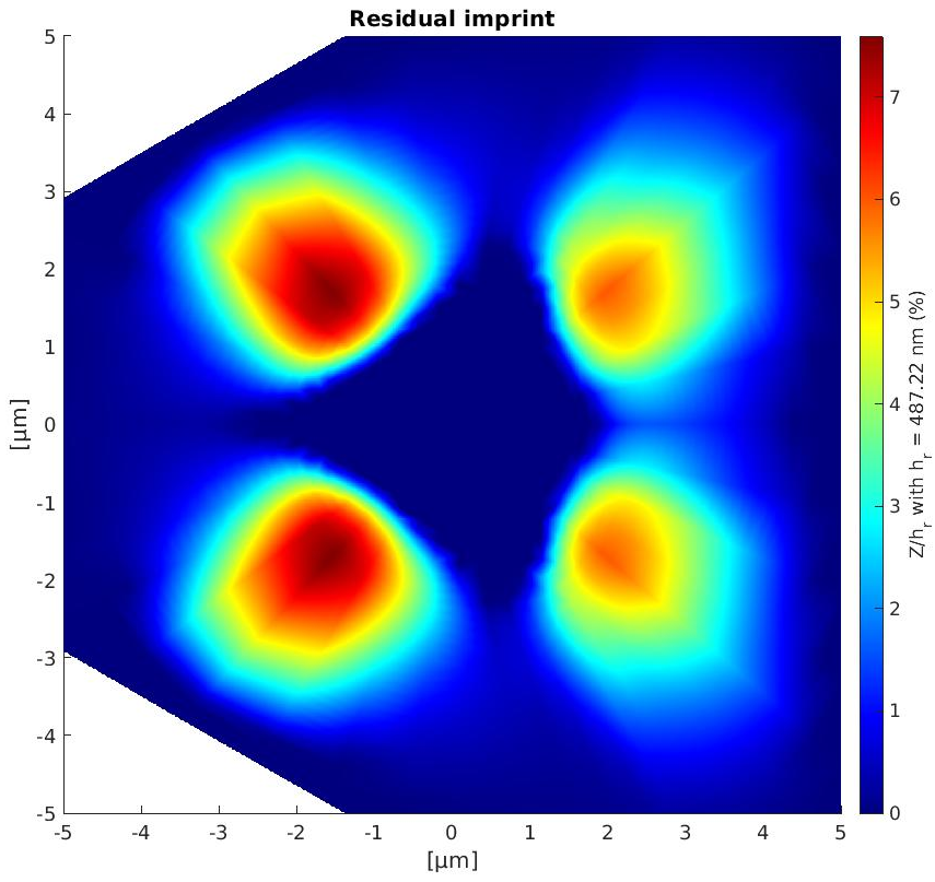
This study has been conducted as part of the the PhD thesis of A.Bourceret (FEMTO) supervised by A.Lejeune, Y.Gaillard and F.Richard (FEMTO). It deals with the modelling of a Berkovich nanoindentation test on a copper sample which is described by the Meric-Cailletaud single crystal law at finite strain.
The imposed displacement of the berkovich indenter to a maximum value of \(500\,nm\). For this simulation the material parameters identified copper by Méric et al were used [1].
The finite element model based contains \(4.10^4\) elements for the geometric description of the copper sample and the Berkovich indenter. This model is treated by the Ansys finite element solver. The results of this simulation are reported on Figure 1 which represents the simulated residual topography.
code_asterBased on this tutorial, Nicolò Grilli (University of Bristol)
published a series of three videos showing in details how to make single
and polycrystal simulations with MFront and
code_aster:
The series adresses several advanced topics regarding the interface between code_ater and MFront:
which can be very handy for a lot of users.