1 Introduction

Constitutive equations for porous (visco-)plasticity are used to perform ductile fracture simulations, adding the porosity as an internal state variable. Porosity evolution is driven by nucleation laws and growth due to plastic flow.

While some implementations of these models based on implicit schemes are already available in MFront (Gurson [1], Gurson-Tvergaard-Needleman [2], …), their numerical treatment have specific issues:

• Phenomenological laws describing porosity nucleation may have threshold to be activated or inhibited.
• Material failure usually happens when the porosity reaches a critical value corresponding to the collapse of the yield surface. Detection of material failure is awkward when the equations governing the porosity evolution are included in the implicit system to be solved. For example, the estimates of the solution may exceed the critical value during the iterations while the solution of the implicit scheme may be below this critical value.

Those issues were previously overcome by considering an explicit treatment of the porosity evolution, which requires small time steps.

The purpose of this work is twofold:

• Propose a robust fully implicit algorithm which can handle thresholds of nucleation laws and material failure.
• Extend the StandardElastoViscoPlasticity brick to this class of behaviours, allowing a declarative syntax similar as:

@Brick "StandardElastoViscoPlasticity" {
   stress_potential : "Hooke" {
      young_modulus : 200e9,
      poisson_ratio : 0.3
   },
   inelastic_flow : "Plastic" {
      criterion : "GursonTvergaardNeedleman" {
         q1 : 1.5,
         q2 : 1.0,
         q3 : 2.2,
         fc : 0.01,
         fr : 0.1
      },
      isotropic_hardening : "Linear" {
         R0 : 150e6
      }
   },
   porosity_evolution : {
      nucleation_model : "Chu_Needleman" {
         An : 0.01,
         pn : 0.1,
         sn : 0.1
      },
      growth_model : "StandardPlasticModel"
};

Note For backward compatibility, effect of the porosity on plastic flows will not be taken into account if no porosity_evolution section is declared.

This document is meant to be part of the MFront documentation. It will be available on the MFront website and on the ResearchGate page of the project. The authors have carefully checked that no unpublished material data has been used in the examples.

1.1 Outline

Section 2 provides a description of several stress criteria of interest for porous (visco-)plasticity and some common nucleation laws.

Section 3 describes two implicit schemes suitable for the integration of the previous constitutive laws:

• The first one is the standard implicit scheme where the implicit equations associated with all the state variables are solved all at once using a Newton-like algorithm.
• The second one is built on a staggered approach in which the porosity evolution and the evolution of the other state variables are solved independently. Both evolutions are repeated until the implicit equations associated with all the state variables are all satisfied. We show that, if required, an exact consistent tangent operator can be derived.

Section 4 discusses the design choices made for the extension of MFront’ StandardElastoViscoPlasticity brick.

Section 5 is devoted to unit tests and verifications.

Section 6 describes early results that proves the robustness of the proposed schemes.

Appendix 8.1 is dedicated to the computation of the stress criterion which may require solving a non linear equation by Newton algorithm.

Appendix 8.2 gives the derivatives of some common nucleation laws.

Appendix 8.3 gives the derivatives of some common porous stress criteria.

Appendix 8.4 describes a regularization of the effective porosity in the Gurson-Tvergaard-Needleman stress criterion.

Appendix 8.5 details some numerical tricks to improve the robustness of finite element simulations performed with Cast3M using the constitutive laws from the extended StandardElastoViscoPlasticity brick.

Appendix 8.6 is dedicated to the description of the various options that can be declared in the porosity_evolution section inside the declaration of the StandardElastoViscoPlasticity brick.

2 General framework

In the framework adopted in this report, a porous plastic model is defined by a stress criterion \(\sigma_{\star}\) which depends explicitly on the stress tensor \(\underline{\sigma}\) and the porosity \(f\):

\[ \sigma_{\star}= \phi(\underline{\sigma},f) \]

This stress criterion is used to define the yield surface or the intensity of the viscoplastic flow.

Concerning the flow rule, two main classes of models are classically found in the literature. In the first class of model, the porosity does not change the expression of the flow rule:

\[ \underline{\dot{\varepsilon}}^{\mathrm{p}}= \dot{\lambda}\, {\displaystyle \frac{\displaystyle \partial \sigma_{\star}}{\displaystyle \partial \underline{\sigma}}} = \dot{p}\, {\displaystyle \frac{\displaystyle \partial \sigma_{\star}}{\displaystyle \partial \underline{\sigma}}} \]

i.e. the equivalent (visco-)plastic strain \(p\) is defined as the macroscopic equivalent (visco-)plastic strain and can still be identified as the plastic multiplier \(\lambda\).

This class of models encompasses:

• the work of Ponte-Castaneda (see [3]), which is the theorical basis of several viscoplastic behaviours used in uranium dioxyde fuels [4, 5];
• the work of Rousselier [6].

In the second class, the flow rule is affected by a correction factor \(1-f\) (see [7]):

\[ \underline{\dot{\varepsilon}}^{\mathrm{p}}= \dot{\lambda}\, {\displaystyle \frac{\displaystyle \partial \sigma_{\star}}{\displaystyle \partial \underline{\sigma}}} = (1 - f)\, \dot{p}\, {\displaystyle \frac{\displaystyle \partial \sigma_{\star}}{\displaystyle \partial \underline{\sigma}}} \]

where \(f\) is the porosity. Here, \(p\) can be identified to the equivalent (visco-)plastic strain in the matrix and it is no more equal to the plastic multiplier \(\lambda\).

Note

The term \((1-f)\) comes from the definition of \(p\) as the equivalent plastic strain in the matrix through the modelling of hardening:

\[ \displaystyle{\underline{\sigma}:\underline{\dot{\varepsilon}}^{\mathrm{p}}= \dot{\lambda} \underline{\sigma}\, \colon\,{\displaystyle \frac{\displaystyle \partial \sigma_{\star}}{\displaystyle \partial \underline{\sigma}}}} = \dot{\lambda} \sigma_{\star}= (1 - f)R(p) \dot{p} \Rightarrow \dot{\lambda} = (1 - f) \dot{p} \]

where \(R{\left(p\right)}\) is the radius of the yield surface.

The evolution of porosity is composed of two terms: one due to plastic flow and another one due to nucleation \(A_n^i dp\):

\[\dot{f} = (1 - f){\mathrm{tr}{\left(\underline{\dot{\varepsilon}}^{\mathrm{p}}\right)}} + \sum_j A_n^j \dot{p}\]

The first term describes the incompressibility of the matrix under the assumption that the change of volume associated with the elastic part of the strain is negligible. This assumption is common, although adding the elastic contribution is fairly easy, see Section 3.1.1.

2.1 Stress criteria

Different stress criteria implemented in the brick are described below.

• Gurson-Tvergaard-Needleman [2]

\[ S = {\left(\dfrac{\sigma_{vM}}{\sigma_{\star}} \right)}^2 + 2 q_1 f_{\star} \cosh{{\left(\dfrac{3}{2} q_2 \dfrac{\sigma_m}{\sigma_{\star}} \right)}} - 1 - q_3 f_{\star}^2 = 0 \qquad(1)\] which defines implicitly \(\sigma_{\star}\), where \(\sigma_{vM}\) is the von Mises equivalent stress, and \(\sigma_m\) the mean stress. \(f_{\star}\) is defined such that:

\[ f_{\star} = \left\{ \begin{array}{ll} \delta f & \mbox{if } f < f_c \\ f_c + \delta (f - f_c) & \mbox{otherwise} \end{array} \right. \] and: \[ \delta = \left\{ \begin{array}{ll} 1 & \mbox{if } f < f_c \\ \dfrac{f_u- f_c }{f_r - f_c} & \mbox{otherwise} \end{array} \right. \] where \(f_{u}\) is the root of \(2\,q_1\,f-1-q_3\,f^{2}\).

The parameters of the model are:

\[\left\{q_1,q_2,q_3,f_c,f_r \right\} \]

For \(\left\{q_1,q_2,q_3,f_c,f_r \right\} = \left\{1,1,1,+\infty,-\right\}\), Gurson-Tvergaard-Needleman model reduces to the Gurson model [1] which has no free parameter.

Note that the physical meaning of \(q_3\) different from \(q_1^2\) is doubtful. Moreover, the current implementation is incorrect for \(q_3 > q_1^2\).

• Rousselier-Tanguy-Besson [8]

\[ S = \dfrac{\sigma_{vM}}{(1- f )\sigma_{\star}} + \dfrac{2}{3} f D_R \exp{{\left(\dfrac{3}{2} q_R \dfrac{\sigma_m}{(1 - f )\sigma_{\star}} \right)}} - 1 = 0 \qquad(2)\]

The effective stress \(\sigma_{\star}\) which is solution of this equation is:

\[\sigma_{\star}= \dfrac{q_R \sigma_{vM}}{(1 - f) {\left(q_R - \dfrac{2}{3T}L{\left(q_R D_R f T \exp{{\left(\dfrac{3}{2} q_R T\right)}}\right)}\right)}} \]

where \(L\) is the Lambert function, and \(T = \sigma_m / \sigma_{vM}\) the stress triaxiality. The parameters of the model are:

\[\left\{q_R,D_R \right\} \]

2.2 Nucleation terms

Different nucleation terms are available and are described below. Multiple nucleation terms can be used simultaneously.

• Chu-Needleman strain based [9]

\[ A_n = \dfrac{f_N}{s_N \sqrt{2\pi}} \exp{{\left(-\dfrac{1}{2} {\left(\dfrac{p - \epsilon_N}{s_N} \right)}^2 \right)} } \qquad(3)\]

where \(\{f_N,s_N,\epsilon_N\}\) are material parameters, and \(p\) is the matrix equivalent plastic strain.

• Chu-Needleman stress based [9]

\[ A_n = \dfrac{f_N}{s_N \sqrt{2\pi}} \exp{{\left(-\dfrac{1}{2} {\left(\dfrac{\sigma_I - \sigma_N}{s_N} \right)}^2 \right)} } \]

where \(\{f_N,s_N,\sigma_N\}\) are material parameters, and \(\sigma_I\) is the maximal positive principal stress.

• Power-Law strain based

\[ A_n = f_N \left<\dfrac{p}{\epsilon_N} - 1 \right>^m \quad \mathrm{if}\quad \int A_n dp \leq f_{\mathrm{nuc}}^{max} \qquad(4)\]

where \(\{f_N,m,\epsilon_N,f_{\mathrm{nuc}}^{max} \}\) are material parameters, \(p\) is the matrix equivalent plastic strain. In the previous expression, \(\left<.\right>\) denotes the Macaulay bracket, i.e. positive part of a number:

\[ \left<x\right> = \max{\left(x,0\right)} \]

• Power-Law stress based

\[ A_n = f_N \left<\dfrac{\sigma_I}{\sigma_N} - 1 \right>^m \quad \mathrm{if}\quad \int A_n dp \leq f_{\mathrm{nuc}}^{max} \]

where \(\{f_N,m,\sigma_N,f_{\mathrm{nuc}}^{max}\}\) are material parameters, and \(\sigma_I\) is the maximal positive principal stress.

3 Implicit schemes

This section is devoted to the presentation of two implicit schemes that may be used to integrate the constitutive equations presented in Section 2.

3.1 Standard implicit scheme

Assuming a single porous stress criterion whose flow is modified by the porosity evolution, the constitutive equations lead to the following system to be solved for an elastoplastic evolution:

\[ \begin{aligned} \underline{\dot{\varepsilon}}^{\mathrm{el}}+ \underline{\dot{\varepsilon}}^{\mathrm{p}}- \underline{\dot{\varepsilon}}^{\mathrm{to}}&= 0 \\ \sigma_{\star}- R(p) &= 0 \\ \dot{f} - (1 - f){\mathrm{tr}{\left(\underline{\dot{\varepsilon}}^{\mathrm{p}}\right)}} - \sum_j A_n^j \dot{p} &=0 \end{aligned} \qquad(5)\]

This system must be closed by adding the relation between the stress \(\underline{\sigma}\) and the elastic strain \(\underline{\varepsilon}^{\mathrm{el}}\). In the report, we assume that the standard Hooke law holds:

\[ \underline{\sigma}= \underline{\underline{\mathbf{D}}}\,\underline{\varepsilon}^{\mathrm{el}} \]

where \(\underline{\underline{\mathbf{D}}}\) is the elastic stiffness tensor.

A semi-implicit method is used to solve these equations according to the variables \(\{\Delta\,\underline{\varepsilon}^{\mathrm{el}}, \Delta\,p, \Delta\,f \}\)

\[ \mathcal{R}{\left(\Delta\,\underline{\varepsilon}^{\mathrm{el}}, \Delta\,p, \Delta\,f\right)}=0 \qquad(6)\]

The residual \(\mathcal{R}\) can be decomposed by blocks as follows:

\[ \begin{aligned} \mathcal{R}_{\Delta\,\underline{\varepsilon}^{\mathrm{el}}} = \Delta\,\underline{\varepsilon}^{\mathrm{el}}+ (1 - {\left.f\right|_{t+\theta\,\Delta\,t}}) \Delta\,p \, {\left.{\displaystyle \frac{\displaystyle \partial \sigma_{\star}}{\displaystyle \partial \underline{\sigma}}}\right|_{t+\theta\,\Delta\,t}} - \Delta\,\underline{\epsilon}_{to} &= 0 \\ \mathcal{R}_{\Delta\,p} = \sigma_{\star}- R({\left.p\right|_{t+\theta\,\Delta\,t}}) &= 0 \\ \mathcal{R}_{\Delta\,f} = \Delta\,f - (1 - {\left.f\right|_{t+\theta\,\Delta\,t}})^2 \Delta\,p \, {\mathrm{tr}{\left({\left.{\displaystyle \frac{\displaystyle \partial \sigma_{\star}}{\displaystyle \partial \underline{\sigma}}}\right|_{t+\theta\,\Delta\,t}}\right)}} - \sum_j {\left.A_n^j\right|_{t+\theta\,\Delta\,t}}\,\Delta\,p &=0 \end{aligned} \qquad(7)\]

In the previous equation, \(\theta\) is a numerical parameter (\(\theta\in[0:1]\)).

Solving this system using a Newton-Raphson algorithm requires computing the Jacobian matrix:

\[ J= \begin{pmatrix} \begin{array}{lll} {\displaystyle \frac{\displaystyle \partial \mathcal{R}_{\Delta\,\underline{\varepsilon}^{\mathrm{el}}}}{\displaystyle \partial \Delta\,\underline{\varepsilon}^{\mathrm{el}}}} & {\displaystyle \frac{\displaystyle \partial \mathcal{R}_{\Delta\,\underline{\varepsilon}^{\mathrm{el}}}}{\displaystyle \partial \Delta\,p}} & {\displaystyle \frac{\displaystyle \partial \mathcal{R}_{\Delta\,\underline{\varepsilon}^{\mathrm{el}}}}{\displaystyle \partial \Delta\,f}} \\ {\displaystyle \frac{\displaystyle \partial \mathcal{R}_{\Delta\,p}}{\displaystyle \partial \Delta\,\underline{\varepsilon}^{\mathrm{el}}}} & {\displaystyle \frac{\displaystyle \partial \mathcal{R}_{\Delta\,p}}{\displaystyle \partial \Delta\,p}} & {\displaystyle \frac{\displaystyle \partial \mathcal{R}_{\Delta\,p}}{\displaystyle \partial \Delta\,f}} \\ {\displaystyle \frac{\displaystyle \partial \mathcal{R}_{\Delta\,f}}{\displaystyle \partial \Delta\,\underline{\varepsilon}^{\mathrm{el}}}} & {\displaystyle \frac{\displaystyle \partial \mathcal{R}_{\Delta\,f}}{\displaystyle \partial \Delta\,p}} & {\displaystyle \frac{\displaystyle \partial \mathcal{R}_{\Delta\,f}}{\displaystyle \partial \Delta\,f}} \\ \end{array} \end{pmatrix} \qquad(8)\]

where the different terms can be written as [7]:

\[ \begin{aligned} {\displaystyle \frac{\displaystyle \partial \mathcal{R}_{\Delta\,\underline{\varepsilon}^{\mathrm{el}}}}{\displaystyle \partial \Delta\,\underline{\varepsilon}^{\mathrm{el}}}} &= \underline{\underline{\mathbf{I}}} + \theta \Delta\,p \; \bigg(1 - {\left.f\right|_{t+\theta\,\Delta\,t}}\bigg) {\left.\dfrac{\partial^2 \sigma_{\star}}{\partial \underline{\sigma}^2}\right|_{t+\theta\,\Delta\,t}}\,\colon\,{\left.{\underline{\underline{\mathbf{D}}}}\right|_{t+\theta\,\Delta\,t}} \\ {\displaystyle \frac{\displaystyle \partial \mathcal{R}_{\Delta\,\underline{\varepsilon}^{\mathrm{el}}}}{\displaystyle \partial \Delta\,p}} &= \bigg(1 - {\left.f\right|_{t+\theta\,\Delta\,t}}\bigg) {\left.{\displaystyle \frac{\displaystyle \partial \sigma_{\star}}{\displaystyle \partial \underline{\sigma}}}\right|_{t+\theta\,\Delta\,t}} \\ {\displaystyle \frac{\displaystyle \partial \mathcal{R}_{\Delta\,\underline{\varepsilon}^{\mathrm{el}}}}{\displaystyle \partial \Delta\,f}} &= \theta \Delta\,p \; \bigg( \bigg(1 - {\left.f\right|_{t+\theta\,\Delta\,t}}\bigg)\, {\left.\dfrac{\partial^2 \sigma_{\star}}{\partial \underline{\sigma}\partial f}\right|_{t+\theta\,\Delta\,t}} - {\left.{\displaystyle \frac{\displaystyle \partial \sigma_{\star}}{\displaystyle \partial \underline{\sigma}}}\right|_{t+\theta\,\Delta\,t}} \bigg) \\ {\displaystyle \frac{\displaystyle \partial \mathcal{R}_{\Delta\,p}}{\displaystyle \partial \Delta\,\underline{\varepsilon}^{\mathrm{el}}}} &= \theta \; {\left.{\displaystyle \frac{\displaystyle \partial \sigma_{\star}}{\displaystyle \partial \underline{\sigma}}}\right|_{t+\theta\,\Delta\,t}}\,\colon\,{\left.{\underline{\underline{\mathbf{D}}}}\right|_{t+\theta\,\Delta\,t}} \\ {\displaystyle \frac{\displaystyle \partial \mathcal{R}_{\Delta\,p}}{\displaystyle \partial \Delta\,p}} &= - \theta \; \dfrac{d R(p)}{d p} \\ {\displaystyle \frac{\displaystyle \partial \mathcal{R}_{\Delta\,p}}{\displaystyle \partial \Delta\,f}} &= \theta \; {\displaystyle \frac{\displaystyle \partial \sigma_{\star}}{\displaystyle \partial f}} |_{t+\theta \Delta\,t} \\ {\displaystyle \frac{\displaystyle \partial \mathcal{R}_{\Delta\,f}}{\displaystyle \partial \Delta\,\underline{\varepsilon}^{\mathrm{el}}}} &= - \theta \; \Delta\,p \; \bigg(1 - {\left.f\right|_{t+\theta\,\Delta\,t}}\bigg)^2 \; \bigg({\left.\dfrac{\partial^2 \sigma_{\star}}{\partial \underline{\sigma}^2}\right|_{t+\theta\,\Delta\,t}}\,\colon\,{\left.{\underline{\underline{\mathbf{D}}}}\right|_{t+\theta\,\Delta\,t}}\bigg)\,\colon\,\underline{I} - \theta \Delta\,p \sum_j {\left.{\displaystyle \frac{\displaystyle \partial A_n^j}{\displaystyle \partial \underline{\sigma}}}\right|_{t+\theta\,\Delta\,t}}\,\colon\,{\left.{\underline{\underline{\mathbf{D}}}}\right|_{t+\theta\,\Delta\,t}} \\ {\displaystyle \frac{\displaystyle \partial \mathcal{R}_{\Delta\,f}}{\displaystyle \partial \Delta\,p}} &= - \bigg(1 - {\left.f\right|_{t+\theta\,\Delta\,t}}\bigg)^2 \; {\left.{\displaystyle \frac{\displaystyle \partial \sigma_{\star}}{\displaystyle \partial \underline{\sigma}}}\right|_{t+\theta\,\Delta\,t}}\,\colon\,\underline{I} - \theta \Delta\,p \sum_j {\left.{\displaystyle \frac{\displaystyle \partial A_n^j}{\displaystyle \partial p}}\right|_{t+\theta\,\Delta\,t}} - \sum_j {\left.A_n^j\right|_{t+\theta\,\Delta\,t}} \\ {\displaystyle \frac{\displaystyle \partial \mathcal{R}_{\Delta\,f}}{\displaystyle \partial \Delta\,f}} &= 1 - \theta \; \Delta\,p \; \bigg(1 - {\left.f\right|_{t+\theta\,\Delta\,t}}\bigg) \bigg(-2 \; {\displaystyle \frac{\displaystyle \partial \sigma_{\star}}{\displaystyle \partial \underline{\sigma}}} + \bigg(1 - {\left.f\right|_{t+\theta\,\Delta\,t}}\bigg) \; \dfrac{\partial^2 \sigma_{\star}}{\partial \underline{\sigma}\partial f} \bigg) \underline{I} - \theta \Delta\,p \sum_j {\left.{\displaystyle \frac{\displaystyle \partial A_n^j}{\displaystyle \partial f}}\right|_{t+\theta\,\Delta\,t}} \\ \end{aligned} \]

Therefore, the definition of a porous model requires to give the following expressions for the stress criterion \(\sigma_{\star}\):

\[\left\{\sigma_{\star}, {\displaystyle \frac{\displaystyle \partial \sigma_{\star}}{\displaystyle \partial \underline{\sigma}}}, \dfrac{\partial \sigma_{\star}}{\partial f}, \dfrac{\partial^2 \sigma_{\star}}{\partial \underline{\sigma}^2}, \dfrac{\partial^2 \sigma_{\star}}{\partial \underline{\sigma}\partial f} \right\} \]

as well as the following expressions for each nucleation mechanism:

\[ \left\{A_n^i, {\displaystyle \frac{\displaystyle \partial A_n^i}{\displaystyle \partial \underline{\sigma}}}, {\displaystyle \frac{\displaystyle \partial A_n^i}{\displaystyle \partial p}} , {\displaystyle \frac{\displaystyle \partial A_n^i}{\displaystyle \partial f}} \right\} \]

These expressions are detailed for the stress criteria and nucleation formulas currently implemented into the brick in Appendixes 8.2 and 8.3.

3.1.1 Taking the elastic contribution to the porosity growth into account

Adding the elastic contribution to the porosity growth is trivially performed by substracting the following term to the implicit equation associated with the porosity evolution:

\[ \mathcal{R}_{\Delta\,f} \mathrel{-}= {\left(1 - {\left.f\right|_{t+\theta\,\Delta\,t}}\right)}\,{\mathrm{tr}{\left(\Delta\underline{\varepsilon}^{\mathrm{el}}\right)}} \]

The following term must be added to the block \({\displaystyle \frac{\displaystyle \partial \mathcal{R}_{\Delta\,f}}{\displaystyle \partial \Delta\,f}}\):

\[ {\displaystyle \frac{\displaystyle \partial \mathcal{R}_{\Delta\,f}}{\displaystyle \partial \Delta\,f}} \mathrel{+}= \theta\,{\mathrm{tr}{\left(\Delta\underline{\varepsilon}^{\mathrm{el}}\right)}} \]

And the following term must be added to the block \({\displaystyle \frac{\displaystyle \partial \mathcal{R}_{\Delta\,f}}{\displaystyle \partial \Delta\,\underline{\varepsilon}^{\mathrm{el}}}}\):

\[ {\displaystyle \frac{\displaystyle \partial \mathcal{R}_{\Delta\,f}}{\displaystyle \partial \Delta\,\underline{\varepsilon}^{\mathrm{el}}}} \mathrel{+}= -{\left(1 - {\left.f\right|_{t+\theta\,\Delta\,t}}\right)}\,\underline{I} \]

3.1.2 Special cases for the treatment of the porosity

In the absence of nucleation models and without elastic contribution, the evolution of the porosity is given by the following equation:

\[ \dot{f}={\left(1-f\right)}^{n_{f}}\,\dot{p}\,{\mathrm{tr}{\left(\underline{n}\right)}} \qquad(9)\]

where \(n_{f}\) is equal to:

• \(2\) if the porosity evolution affects the (visco-)plastic flow
• \(1\) if this is not the case.

3.1.2.1 First case (\(n_{f}=1\))

Assuming \(n_{f}=1\), Equation (9) can be integrated by parts:

\[ \int_{{\left.f\right|_{t}}}^{{\left.f\right|_{t+\Delta\,t}}}\dfrac{\mathrm{d}\,u}{1-u}=\log{\left(\dfrac{1-{\left.f\right|_{t}}}{1-{\left.f\right|_{t+\Delta\,t}}}\right)}=\int_{t}^{t+\Delta\,t}\dot{p}\,{\mathrm{tr}{\left(\underline{n}\right)}}\,\mathrm{d}\,t\approx\Delta\,p\,{\mathrm{tr}{\left({\left.\underline{n}\right|_{t+\theta\,\Delta\,t}}\right)}} \]

which leads to the following expression of the increment of the porosity:

\[ \Delta\,f={\left(1-{\left.f\right|_{t}}\right)}\,{\left(1-\exp{\left(-\Delta\,p\,{\mathrm{tr}{\left({\left.\underline{n}\right|_{t+\theta\,\Delta\,t}}\right)}}\right)}\right)} \]

Taking into account the elastic prediction

When taking into account the elastic prediction, the increment of the porosity can be known prior any integration:

\[ \Delta\,f={\left(1-{\left.f\right|_{t}}\right)}\,{\left(1-\exp{\left({\mathrm{tr}{\left(-\Delta\,\underline{\varepsilon}^{\mathrm{to}}\right)}}\right)}\right)} \qquad(10)\]

When applicable, Equation (10), could be very interesting because one can predict the material failure before the material integration. Moreover, removing the evolution of the porosity equation greatly simplifies the resolution of the implicit system.

However, one drawback of this relation is that it introduces the porosity as an implicit function of the increment of the total strain which:

• is incompatible with the assumptions of the StandardElastoViscoPlasticity brick. It thus won’t be treated further in this report;
• complexifies the computation of the consistent tangent operator. In particular, Equation (18), detailed below, is no more valid. However, recent developments of MFront could simplify the computation of the tangent operator in this case, see [10] for details.

Another drawback is that the user would not be able to add its own contribution to the porosity evolution as described in Section 4.2.1.1.

3.1.2.2 Second case (\(n_{f}=2\))

Assuming \(n_{f}=2\), Equation (9) can be integrated by parts:

\[ \int_{{\left.f\right|_{t}}}^{{\left.f\right|_{t+\Delta\,t}}}\dfrac{\mathrm{d}\,u}{{\left(1-u\right)}^{2}}=\dfrac{1}{1-{\left.f\right|_{t}}}-\dfrac{1}{1-{\left.f\right|_{t+\Delta\,t}}}=\int_{t}^{t+\Delta\,t}\dot{p}\,{\mathrm{tr}{\left(\underline{n}\right)}}\,\mathrm{d}\,t\approx\Delta\,p\,{\mathrm{tr}{\left({\left.\underline{n}\right|_{t+\theta\,\Delta\,t}}\right)}} \]

which leads to the following expression of the increment of the porosity:

\[ \Delta\,f={\left(1-{\left.f\right|_{t}}\right)}^{2}\,\dfrac{ \Delta\,p\,{\mathrm{tr}{\left({\left.\underline{n}\right|_{t+\theta\,\Delta\,t}}\right)}} }{ 1+{\left(1-{\left.f\right|_{t}}\right)}\,\Delta\,p\,{\mathrm{tr}{\left({\left.\underline{n}\right|_{t+\theta\,\Delta\,t}}\right)}} } \]

3.1.3 Treatment of bounds on nucleated porosity

Most nucleation models require to set an upper bound \(f_{\mathrm{nuc}}^{j,\max}\) on the maximum nucleated porosity predicted by those models. In this case, the effective nucleated porosity increment is defined as:

\[ \Delta\,f_{n}^{j} = \min{\left({\left.A_n^j\right|_{t+\theta\,\Delta\,t}} \Delta\,p,\,f_{\mathrm{nuc}}^{j,\max}-{\left.f_{n}^{j}\right|_{t}}\right)} \]

This treatment requires that the value of the nucleated porosity at the beginning of the time step is known. Hence it is automatically stored in an auxiliary state variable whatever the value of the save_porosity_increase option passed to the nucleation model.

3.1.4 Specific treatment of strain-based nucleation models

A strain-based nucleation model only depends on the equivalent plastic strain as follows:

\[ {\displaystyle \frac{\displaystyle \mathrm{d}f_{n}^{j}}{\displaystyle \mathrm{d}t}}=A^{j}_{n}{\left(p\right)}\,{\displaystyle \frac{\displaystyle \mathrm{d}p}{\displaystyle \mathrm{d}t}} \qquad(11)\]

See the strain version of the Chu-Needleman nucleation model (Equation (3)) and the strain version of the power-law nucleation model (Equation (4)).

In Equation (7), the contribution of this nucleation model to the implicit equation was set equal to:

\[ \Delta\,f_{n}^{j}\approx A^{j}_{n}{\left({\left.p\right|_{t+\theta\,\Delta\,t}}\right)}\,\Delta\,p \]

However, this is only an approximation.

A more precise estimation can be obtained by integrating Equation (11) by parts, which leads to the following expression of the porosity increment:

\[ \Delta\,f_{n}^{j} = F^{j}_{n}{\left({\left.p\right|_{t+\Delta\,t}}\right)}-F^{j}_{n}{\left({\left.p\right|_{t}}\right)} \qquad(12)\]

where \(F^{j}_{n}\) is one primitive of \(A\), i.e. \(F^{j}_{n}{\left(p\right)}=\displaystyle \int A^{j}_{n}{\left(u\right)}\,\mathrm{d}\,u\). Such a treatment of the nucleated porosity was only considered in [11].

When the function \(A\) also depends on some external state variables, (temperature, fluence), we use the value of those external state variables at the middle of the time step to evaluate the increment of the porosity using Equation (12).

3.1.5 Shortcomings of this implicit scheme

The Newton-Raphson algorithm may fail at finding the solution of the non-linear system of equations, especially when the time step leads to strong increase of the porosity.

Moreover, the porosity evolution leads to specific issues:

• Phenomenological laws describing porosity nucleation may have thresholds to be activated or inhibited.
• Material failure usually happens when the porosity reaches a critical value corresponding to the collapse of the yield surface. Detection of material failure is awkward when the equations governing the porosity evolution are included in the implicit system to be solved. For example, the estimates of the solution may exceed the critical value during the iterations while the solution of the implicit scheme may be below this critical value.

3.2 A staggered approach

As the main convergence issues of the standard implicit scheme are associated with the porosity evolution, we propose in this section a staggered approach where the porosity evolution and the evolution of the other state variables (i.e. the elastic strain \(\underline{\varepsilon}^{\mathrm{el}}\) and the equivalent plastic strain \(p\)) are decoupled. A fixed point algorithm is used to ensure that the increments \(\left\{\Delta\,\underline{\varepsilon}^{\mathrm{el}}, \Delta\,p, \Delta\,f\right\}\) satisfies the Implicit System (7).

3.2.1 Reduced implicit system

Let \(i\) be the current step of the fixed point algorithm. The estimates of the increments of the elastic strain and the equivalent plastic strain at the next iterations, denoted respectively \(\Delta \underline{\varepsilon}^{\mathrm{el}}_{(i+1)}\) and \(\Delta\,p_{(i+1)}\) satisfies a reduced implicit system:

\[ \begin{aligned} \mathcal{R}_{\Delta\,\underline{\varepsilon}^{\mathrm{el}}} = \Delta\,\underline{\varepsilon}^{\mathrm{el}}_{(i+1)} + {\left(1 - f_{(i)}\right)}\,\Delta\,p_{(i+1)}\,{\displaystyle \frac{\displaystyle \partial \sigma_{\star}}{\displaystyle \partial \underline{\sigma}}}{\left(\underline{\varepsilon}^{\mathrm{el}}_{(i+1)},f_{(i)}\right)} - \Delta\,\underline{\epsilon}^{to} &= 0 \\ \mathcal{R}_{\Delta\,p} = \sigma_{\star}{\left(\underline{\varepsilon}^{\mathrm{el}}_{(i+1)},f_{(i)}\right)} - R(p_{(i+1)}) &= 0 \\ \end{aligned} \qquad(13)\]

where:

• \(\underline{\varepsilon}^{\mathrm{el}}_{(i+1)}={\left.\underline{\varepsilon}^{\mathrm{el}}\right|_{t}}+\theta\,\Delta\,\underline{\varepsilon}^{\mathrm{el}}_{(i+1)}\)
• \(p_{(i+1)}={\left.p\right|_{t}}+\theta\,\Delta\,p_{(i+1)}\)
• \(f_{(i)}={\left.f\right|_{t}}+\theta\,\Delta\,f_{(i)}\)

The Implicit System (13) is solved by a standard Newton-Raphson method with the reduced jacobian matrix:

\[ \left[ \begin{array}{lll} {\displaystyle \frac{\displaystyle \partial \mathcal{R}_{\Delta\,\underline{\varepsilon}^{\mathrm{el}}}}{\displaystyle \partial \Delta\,\underline{\varepsilon}^{\mathrm{el}}}} & {\displaystyle \frac{\displaystyle \partial \mathcal{R}_{\Delta\,\underline{\varepsilon}^{\mathrm{el}}}}{\displaystyle \partial \Delta\,p}} \\ {\displaystyle \frac{\displaystyle \partial \mathcal{R}_{\Delta\,p}}{\displaystyle \partial \Delta\,\underline{\varepsilon}^{\mathrm{el}}}} & {\displaystyle \frac{\displaystyle \partial \mathcal{R}_{\Delta\,p}}{\displaystyle \partial \Delta\,p}} \\ \end{array} \right] \qquad(14)\]

Note

In practice, for reasons detailed in Section 3.2.10, we still solve the full Implicit System (7), but the implicit equation is modified as follows:

\[ \mathcal{R}_{\Delta\,f} = \Delta\,f - \Delta\,f_{(i)} \]

3.2.2 Iterative determination of the porosity increment

Letting the constraints on the porosity evolution aside, the porosity is determined iteratively as follows:

\[ \Delta\,f_{(i+1)}^{(uc)} = {\left(1 - f_{(i)}\right)}^2 \Delta\,p_{(i+1)} \, {\mathrm{tr}{\left({\displaystyle \frac{\displaystyle \partial \sigma_{\star}}{\displaystyle \partial \underline{\sigma}}}{\left(\underline{\varepsilon}^{\mathrm{el}}_{(i+1)},f_{(i)}\right)}\right)}} + \sum_{j} A_n^{j}{\left(\underline{\varepsilon}^{\mathrm{el}}_{(i+1)}, p_{(i+1)}, f_{(i)}\right)} \Delta\,p_{(i+1)} \qquad(15)\]

Here the \(\mbox{}^{(uc)}\) superscript means “uncorrected.” Corrections to \(\Delta\,f_{(i+1)}^{(uc)}\) will be introduced in the next paragraphs to deal with thresholds in nucleation laws and detection of material failure.

3.2.3 Treatments of thresholds in nucleation laws

Let:

• \(\Delta \left.f_{n}^{j, (uc)}\right|_{(i+1)}=A_n^{j}{\left(\underline{\varepsilon}^{\mathrm{el}}_{(i+1)}, p_{(i+1)}, f_{(i)}\right)} \Delta\,p_{(i+1)}\) be the uncorrected contribution of the \(j^{\mathrm{th}}\) nucleation law to the porosition evolution.
• \({\left.f_{n}^{j}\right|_{t}}\) be the value of the nucleated porosity due to this nucleation law at the beginning of the time step.
• \(f_{n}^{j, \max{}}\) be the threshold of this nucleation law, i.e. the maximal value of the nucleated porosity due to this law.

\(f_{n}^{j, \max{}}-{\left.f_{n}^{j}\right|_{t}}\) is the maximum allowed increment of the porosity for this nucleation law.

We then define the corrected contribution \(\Delta \left.f_{n}^{j}\right|_{(i+1)}\) as follows:

\[ \Delta \left.f_{n}^{j}\right|_{(i+1)} = \min{\left(\Delta \left.f_{n}^{j, (uc)}\right|_{(i+1)}, f_{n}^{j,\max{}}-{\left.f_{n}^{j}\right|_{t}}\right)} \]

3.2.4 Treatment of material failure

Note

To avoid the introduction of another notation, we still used \(\Delta\,f_{(i+1)}^{(uc)}\) even though corrections related to thresholds in nucleations laws may have been taken into account at this stage.

If \({\left.f\right|_{t}}+\Delta\,f_{(i+1)}^{(uc)}\) is greater than the critical porosity denoted \(\alpha_{1}\,f_{r}\), a dichotomic approach is used:

\[ \Delta\,f_{(i+1)} = \dfrac{1}{2}{\left(f+\Delta\,f_{(i)} + \alpha_{1}\, f_r\right)} - {\left.f\right|_{t}}; \]

This approach allows the porosity to approach the critical porosity smoothly.

The \(\alpha_{1}\) factor is a user defined parameter, chosen equal by default to \(98.5\,\%\). The reason for not allowing the porosity be closer to \(f_{r}\) is than the Implicit System (13) becomes very difficult to solve as the yield surfaces collapses.

3.2.5 Stopping criteria

The iterations are stopped when the porosity becomes stationnary, i.e. when:

\[ \left|\Delta\,f_{(i+1)}^{(uc)}-\Delta\,f_{(i)}\right|<\varepsilon_{f} \qquad(16)\]

where the value of \(\varepsilon_{f}\) is a user defined (by default, a stringent value of \(10^{-10}\) is used).

3.2.6 Acceleration algorithm

3.2.6.1 Aitken acceleration (default)

The Iterative Process (15) can be accelerated using the well known Aitken transformation.

The usage of the Aitken acceleration is enabled by default.

3.2.6.2 Relaxation

To avoid spurious oscillations, a relaxation procedure is used:

\[ \Delta\,f_{(i+1)}=\omega\,\Delta\,f_{(i)}+(1 - \omega)\,\Delta\,f_{(i+1)}^{(uc)} \]

where the relaxation coefficient is chosen equal to \(0.5\).

3.2.7 Detection of the material failure (post-processing)

Once the Stopping Condition (16) is satisfied, material failure is detected when the final porosity is above a given threshold \(\alpha_{2}\,f_{r}\), where \(\alpha_{2}\) is a user defined constant chosen equal to \(98\,\%\) by default.

When the material failure is detected, the value of the auxiliary state variable broken is set to one.

3.2.8 Discussion on the performance of the staggered approach

From a performance point of view, this staggered approach seems a priori less efficient than the standard implicit scheme because the reduced integration scheme will be solved once per iteration of the fixed point algorithm.

The staggered approach is however thought to be more robust, although we do not have performed an in-depth comparison of both monolithic and staggered approaches yet.

It shall also be noted that the number of iterations of the reduced integration implicit system is not proportional to the number of iterations of the fixed point algorithm. Indeed, the solution of the reduced implicit system obtained at the previous iteration of the fixed point algorithm can be used as the starting point of the current resolution of the reduced implicit system. Numerical experiments shows that this strategy is very effective and that close to convergence of the fixed point algorithm the number of iterations required to solve the reduced implicit system is low, i.e. only 2 or 3 iterations are required.

3.2.9 Access to the number of the iterations of the staggered scheme

The variable staggered_scheme_iteration_counter holds the number of iterations of the staggered scheme. One can save this variable in a auxiliary state variable as follows:

//! number of iterations of the staggered scheme at convergence
@AuxiliaryStateVariable real niter;
niter.setEntryName("StaggeredSchemeIterationCounter");

....

@UpdateAuxiliaryStateVariables{
  niter = staggered_scheme_iteration_counter;
}

The total number of evaluations of the implicit scheme is a bit trickier to save. It can be done as follows:

//! number of iterations of the implicit scheme
@AuxiliaryStateVariable real neval;
neval.setEntryName("NumberOfEvaluationOfTheImplicitScheme");

...

@InitLocalVariables{
  ...
  neval = 0;
}

...

@Integrator{
 ++neval;
}

Note

If local sub-stepping is allowed, those two numbers will only reflect the number of iterations and number of evaluations of the last step.

3.2.10 Implementation details and computation of the exact consistent tangent operator

3.2.10.1 Implementation, the @AdditionalConvergenceChecks code block

As depicted on Figure 1, each iteration of the implicit algorithm are decomposed in three steps:

• Updating the stress in the @ComputeStress code block. This code block is automatically handled by the brick.
• Building the residual \(\mathcal{R}\) and the jacobian matrix \(J\) in the @Integrator code block.
• Additional convergence checks in the @AdditionalConvergenceChecks code block. Additional here means that MFront has already checked the convergence of the resolution of implicit scheme using a built-in criterion. This code block may be used to implement a status algorithm which allows activating and/or desactivating some (visco-)plastic flows (see [12]). Here, it is used to implement the staggered approach described in this section.

3.2.10.2 Computation of the exact consistent tangent operator

As described in [10], the consistent tangent operator may be deduced for the jacobian of Implicit System (7) as follows:

\[ {\displaystyle \frac{\displaystyle \mathrm{d}\underline{\sigma}}{\displaystyle \mathrm{d}\Delta\,\underline{\varepsilon}^{\mathrm{to}}}}= {\left.\underline{\underline{\mathbf{D}}}\right|_{t+\Delta\,t}}\,\cdot\,{\displaystyle \frac{\displaystyle \partial \underline{\varepsilon}^{\mathrm{el}}}{\displaystyle \partial \Delta\,\underline{\varepsilon}^{\mathrm{to}}}} \qquad(17)\]

where \({\displaystyle \frac{\displaystyle \partial \underline{\varepsilon}^{\mathrm{el}}}{\displaystyle \partial \Delta\,\underline{\varepsilon}^{\mathrm{to}}}}\) can be determined by solving the following systems of linear equations:

\[ J\,\cdot\,{\displaystyle \frac{\displaystyle \partial \underline{\varepsilon}^{\mathrm{el}}}{\displaystyle \partial \Delta\,\underline{\varepsilon}^{\mathrm{to}}}}=-{\displaystyle \frac{\displaystyle \partial \mathcal{R}}{\displaystyle \partial \Delta\,\underline{\varepsilon}^{\mathrm{to}}}} \]

where \({\displaystyle \frac{\displaystyle \partial \mathcal{R}}{\displaystyle \partial \Delta\,\underline{\varepsilon}^{\mathrm{to}}}}\) have this simple matrix form (in \(3D\)):

\[ {\displaystyle \frac{\displaystyle \partial \mathcal{R}}{\displaystyle \partial \Delta\,\underline{\varepsilon}^{\mathrm{to}}}}=- \begin{pmatrix} 1& 0 & 0 & 0& 0 &0 \\ 0& 1& 0 & 0& 0 &0 \\ 0& 0 & 1 & 0& 0 &0 \\ 0& 0 & 0 & 1& 0 &0 \\ 0& 0 & 0 & 0& 1 &0 \\ 0& 0 & 0 & 0& 0 &1\\ 0& 0 & 0 & 0& 0 &0 \\ \vdots & \vdots & \vdots & \vdots & \vdots & \vdots\\ 0& 0 & 0 & 0& 0 &0 \\ \end{pmatrix} \qquad(18)\]

It would cumbersome to compute the jacobian of the Reduced System (13) during the resolution and then to compute the jacobian of the Full System (7) after convergence for the computation of the consistent tangent operator:

• it would require a significant amount of boiler plate code to define the jacobian matrix for the full implicit system and appropriate views of its blocks (see Equation (8));
• it would require a partial duplication of the code computing the blocks of the jacobian of the reduced implicit system (See Equations (8) and (14)).

We thus rely on a simple trick. We define a flag which is set to true during the iterations of the fixed point algorithm. If this flag is true, the implicit equation of the Full Implicit System (7) is replaced by:

\[ \mathcal{R}_{\Delta\,f} = \Delta\,f - \Delta\,f_{(i)} \]

where \(\Delta\,f_{(i)}\) is the current estimation given by the fixed point algorithm.

This new equation is trivially solved so that the solutions of this modified system do verify the Reduced Implicit System (13). Once the fixed point algorithm has converged, one may simply set the flag to false and build the jacobian matrix (8) of the Full Implicit System (7) by calling the assembly of the implicit scheme once and finally apply Equation (17).

A few things may be noted:

• the overhead implied by this trick seems a priori limited;
• one can easily recover the standard implicit scheme;
• one can easily choose to treat the porosity explicitly.

4 Design choices

4.1 Enrichment of the StressCriterion and InelasticFlow interfaces

The InelasticFlow interface is used by the StandardElastoViscoPlasticity brick to handle inelastic flows. It uses the StressCriterion interface to describe it stress criterion and, for non-associated flows, its flow criterion.

For the brick to properly treat inelastic flows coupled with porosity, a new method called isCoupledWithPorosity- Evolution has been added to those interface. This method returns a boolean value and does not take any argument.

For inelastic flows, the default implementation of the isCoupledWithPorosityEvolution, declared in the In- elasticFlowBase class, returns true if its stress criterion or if its flow criterion (if any) declares to be coupled with the porosity evolution.

The isCoupledWithPorosityEvolution of a stress criterion must return true if and only if the expression of the stress criterion explicitly depends on the porosity.

Note

Implicitly, the brick expects that a stress criterion coupled with porosity is not deviatoric, i.e., that this stress criterion contributes to the porosity growth. The isNormalDeviatoric method of such a stress criterion must return true. This is checked in the InelasticFlowBase class.

As discussed in the introduction, a stress criterion can lead to a correction of the flow rule by a factor \(1-f\). The class StressCriterion now has a method called getPorosityEffectOnEquivalentPlasticStrain which return one of the two following values:

• NO_POROSITY_EFFECT_ON_EQUIVALENT_PLASTIC_STRAIN
• STANDARD_POROSITY_CORRECTION_ON_EQUIVALENT_PLASTIC_STRAIN

4.2 Conditions for the brick to contribute to the porosity evolution

The evolution of the porosity is taken into account:

• if a nucleation model is declared;
• if one stress inelastic flow declares being coupled with the porosity evolution, i.e. that its stress criterion or its flow criterion is coupled with the porosity evolution;
• if the porosity_evolution section is explicitly declared, even if empty.

For example, this declaration will automatically lead to a porosity growth:

@Brick StandardElastoViscoPlasticity{
  stress_potential : "Hooke" {
    young_modulus : 150.e3,
    poisson_ratio : 0.3
  },
  inelastic_flow : "Plastic" {
    criterion : "Gurson1975" {},
    isotropic_hardening : "Linear" {R0 : "0"}
  }
};

Note

It is important to note that, by default (if none of the three above conditions are met), no contribution to the porosity growth will be taken into account, even if the flow direction has an hydrostatic component. For example, the following declaration will not lead to any porosity growth:

@Brick StandardElastoViscoPlasticity{
  stress_potential : "Hooke" {
    young_modulus : 150.e3,
    poisson_ratio : 0.3
  },
  inelastic_flow : "Plastic" {
    criterion : "MohrCoulomb" {
      c : 3.e1,      // cohesion
      phi : 0.523598775598299,    // friction angle angle
      lodeT : 0.506145483078356,  // transition angle (Abbo and Sloan)
      a : 1e1       // tension cuff-off parameter
    },
    isotropic_hardening : "Linear" {R0 : "0"}
  }
};

However, this declaration will lead to a porosity growth:

@Brick StandardElastoViscoPlasticity{
  stress_potential : "Hooke" {
    young_modulus : 150.e3,
    poisson_ratio : 0.3
  },
  inelastic_flow : "Plastic" {
    criterion : "MohrCoulomb" {
      c : 3.e1,      // cohesion
      phi : 0.523598775598299,    // friction angle angle
      lodeT : 0.506145483078356,  // transition angle (Abbo and Sloan)
      a : 1e1       // tension cuff-off parameter
    },
    isotropic_hardening : "Linear" {R0 : "0"}
  }
  porosity_evolution: {}
};

The porosity_evolution section has a significant importance in this document. The various options that can be declared in this section are described in Appendix 8.6.

4.2.0.1 Declaration of the porosity as a state variable (if required)

If the evolution of the porosity is taken into account, a state variable called f with the glossary name Porosity is automatically declared if no state variable with this glossary name has been declared. In the latter case, this variable is used (and updated) by the brick.

This choice allows the user to easily add new nucleation model or to add a new inelastic flow coupled with porosity by adding the appropriate state variables and adding the associated implicit equations in the @Integrator code block.

For example, assuming that the staggered approach described in Section 3.2 is used, one may add the contribution of the solid swelling as follows:

@ExternalStateVariable real ss;
ss.setGlossaryName("SolidSwelling");

@Brick StandardElastoViscoPlasticity{
  stress_potential : "Hooke" {
    young_modulus : 150.e3,
    poisson_ratio : 0.3
  },
  inelastic_flow : "Plastic" {
    criterion : "Gurson1975" {},
    isotropic_hardening : "Linear" {R0 : "0"}
  }
};

@Integrator{
  // adding the contribution of the solid swelling
  // the porosity increase in the implicit equation describing
  // the porosity.
  // This shall only been done after the convergence of the
  // staggered scheme has converged.
  if(compute_standard_system_of_implicit_equations){
    ff -= ;
  }
}

@AdditionalConvergenceChecks {
  // adding the contribution of the solid swelling
  // the porosity increase to the next extimate of the porosity by
  // the staggered scheme.
  // This shall only been done after the convergence of the
  // staggered scheme has converged.
  if (converged && (!compute_standard_system_of_implicit_equations)) {
    next_estimate_of_the_porosity_increment += ...
  }
}

The previous code uses variables that are automatically defined by the StandardElastoViscoPlasticity brick when the staggered approach is used:

• compute_standard_system_of_implicit_equations is a boolean value which is false until the staggered scheme converges;
• next_estimate_of_the_porosity_increment is a variable only accessible in the @AdditionalCon- vergenceChecks block which must hold the next estimate of the porosity increment. This variable is automatically initialized to zero.

Other variables automatically defined by the StandardElastoViscoPlasticity brick may be helpful to couple constitutive equations with user defined ones:

• in the @InitLocalVariables code block, the upper_bound_of_the_porosity variable may be updated by the user to change the value of the upper bound of the porosity as follows:

    upper_bound_of_the_porosity = min(upper_bound_of_the_porosity, 
                                      .... // user_defined_bound
                                      );

• in the @AdditionalConvergenceChecks code block, the fixed_point_converged boolean variable might be used add other convergence criteria to the staggered algorithm, as follows:

    if (converged && (!compute_standard_system_of_implicit_equations)) {
      fixed_point_converged = ....
    }

4.3 Effect of the porosity on the equivalent strain definition

By default, the value returned by the getPorosityEffectOnEquivalentPlasticStrain method of the stress criterion is used to decipher if the porosity affects definition of the equivalent plastic strain and the flow rule.

However, this may be changed by specifying the porosity_effect_on_equivalent_plastic_strain option in the definition of the inelastic flow. Valid strings are StandardPorosityEffect (or equivalently " standard_- porosity_effect) or None (or equivalently none or false).

4.4 Saving individual contributions to the porosity evolutions in dedicated auxiliary state variables

The porosity evolves either due to nucleation or growth. For post-processing reasons, it may be worth to distinguish those contributions in dedicated auxiliary state variables. However, for performance reasons (mostly because additional auxiliary state variables implied a memory overhead), this shall not be the default choice.

The brick allows the user to specify if those additional variables shall be defined for all mechanisms in the porosity- _evolution section as follows:

  porosity_evolution: {
    save_individual_porosity_increase: true
  }

However, this behaviour can be overloaded in every inelastic flow section and every nucleation model by setting the save_porosity_increase boolean variable.

For example, one may use the following declaration:

  inelastic_flow : "Plasticity" {
    criterion : "Gurson1975",
    isotropic_hardening : "Voce" {R0 : 200, Rinf : 100, b : 20},
    save_porosity_increase : true
  }

Note

Inelastic flows which declare that the flow is deviatoric discard those options and never declare an auxiliary state variable associated with the porosity growth.

4.5 Taking into account the elastic contribution in the porosity growth

By default, the elastic contribution in the porosity growth is not taken into account.

This could be changed by setting the elastic_contribution options to true as follows:

   porosity_evolution: {
    elastic_contribution: true
  }

5 Verifications

The stress criteria implemented are verified by comparing the results obtained through MTest simulations to reference solutions. Axisymmetric loading conditions are considered under small strains settings:

\[ \underline{\sigma} = \sigma \begin{pmatrix} 1 & 0 & 0 \\ 0 & A & 0\\ 0 & 0 & A \end{pmatrix} \]

A typical MTest file used for these simulations is shown below:

@ModellingHypothesis 'Tridimensional';
@Behaviour<Generic> 'src/libBehaviour.so' 'GTN';
@InternalStateVariable 'Porosity' 1e-3;
@ExternalStateVariable 'Temperature' 293.15 ;

@Real 'A' '0.4';
@NonLinearConstraint<Stress> 'SYY - A*SXX';
@NonLinearConstraint<Stress> 'SZZ - A*SXX';

@ImposedStrain 'EXX' {0 : 0, 1 : 0.5};
@Times{0, 1. in 1000};

Without hardening, the differential equations governing the evolutions of internal state variables are, for the GTN model: \[ \begin{aligned} \frac{d \varepsilon_{yy}^p}{d \varepsilon_{xx}^p} &= \frac{q_1 q_2 f_{\star}\sinh{{\left(\dfrac{1}{2} q_2 (1+2\alpha) \dfrac{\sigma}{\sigma_0}\right)}} + \dfrac{\sigma}{\sigma_0}(\alpha - 1)}{q_1 q_2 f_{\star}\sinh{{\left(\dfrac{1}{2} q_2 (1+2\alpha) \dfrac{\sigma}{\sigma_0}\right)}} + 2\dfrac{\sigma}{\sigma_0}(1 - \alpha )} \ \ \ \ \ \mathrm{with} \ \ \ \ \ S(\sigma,f) = 0\\ \frac{df}{d \varepsilon_{xx}^p} &= (1 - f)\left(1+ 2 \frac{d \varepsilon_{yy}^p}{d \varepsilon_{xx}^p} \right) \end{aligned} \] The same equations also hold for the Gurson model with \((q_1,q_2,f_{\star}) = (1,1,f)\). For the Rousselier model, the equations are: \[ \begin{aligned} \frac{d \varepsilon_{yy}^p}{d \varepsilon_{xx}^p} &= \frac{D_R q_R f\exp{{\left(\dfrac{1}{2} \dfrac{q_R}{1-f} (1+2\alpha) \dfrac{\sigma}{\sigma_0}\right)}} - 1.5}{D_R q_R f\exp{{\left(\dfrac{1}{2} \dfrac{q_R}{1-f} (1+2\alpha) \dfrac{\sigma}{\sigma_0}\right)}} + 3} \ \ \ \ \ \mathrm{with} \ \ \ \ \ S(\sigma,f) = 0\\ \frac{df}{d \varepsilon_{xx}^p} &= (1 - f)\left(1+ 2 \frac{d \varepsilon_{yy}^p}{d \varepsilon_{xx}^p} \right) \end{aligned} \] These differential equations are solved with respect to \(\varepsilon_{xx}^p\) using the ode45 function of the Matlab software, and the stress magnitude \(\sigma\) is computed by solving the stress criteria. Elastic strains are finally added to the plastic strains using Hooke’s law to obtain total strains. These solutions, that can be obtained for arbitrary precision, are the reference solutions to which the results from MTest simulations are compared.

A perfect agreement is obtained between the reference solutions and the MTest results, as depicted on Figure 2, validating the implementation of the equations of these models. Finally, the jacobians of all models have been verified with respect to the numerical jacobian.

6 Applications and Finite Element simulations

6.1 Axisymmetric tensile tests simulations

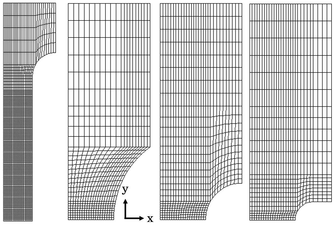
In this scope, the StandardElastoViscoPlasticity brick is tested using the finite elements software Cast3M. The Gurson-Tvergaard-Needleman stress criterion is used to model the ductile failure of Notched Tensile (NT) Samples and Simple Tensile (ST) ones. The \(2D\) meshes are shown on Figure 3 .

The material’s behavior is adapted to aluminum alloys from which the vessel of Fast Neutron Research Reactors are fabricated. The element size is chosen to be \(100\,\mu m\) based on metallurgical studies that take into account the importance of the nucleation phase during damage. The nucleation is modeled by a Stress-based law that is implemented as follows [13] :

\[ A_n = f_N \left<\frac{\sigma_I}{\sigma_N} - 1 \right>^m \ \ \ \ \ \mathrm{if}\ \ p \geq p_N, \ \ \mathrm{and}\ \ \int A_n dp \leq f_{\mathrm{nuc}}^{max} \]

where \(\{f_N, p_N, m,\sigma_N,f_{\mathrm{nuc}}^{max}\}\) are material parameters, and \(\sigma_I\) is the maximum positive principal stress.

Material’s Behavior

@Brick StandardElastoViscoPlasticity{
 stress_potential : "Hooke" {young_modulus : 70e3, poisson_ratio : 0.3},
 inelastic_flow : "Plastic" {
   criterion : "GursonTvergaardNeedleman1982" {
     f_c : 0.04,
     f_r : 0.056,
     q_1 : 2.,
     q_2 : 1.,
     q_3 : 4.
   },
   isotropic_hardening : "Linear" {R0 : 274},
   isotropic_hardening : "Voce" {R0 : 0, Rinf : 85, b : 17},
   isotropic_hardening : "Voce" {R0 : 0, Rinf : 17, b : 262},
   nucleation_model : "Power-based" {
     An0 : 2.92,
     s1_n : 500,
     p_n : 0.0321,
     s1_max : 700,
     fg_max : 0.0215,
     ng : 2
   }
 }

The numerical response of NT specimens (notch radii are noted as : NT10, NT4, and NT2) is shown on Figure 4 and compared to the experimental results.

One can see that the numerical convergence is rather good at the crack initiation phase where the reaction force decreases suddenly. Some aspects could be improved regarding the plastic flow and the damage parameters to smoothly follow the crack propagation modelled by the sudden force drop. Such improvements depends on the finite element solver used and must not be confused with the robustness of the StandardElastoViscoPlasticity brick.

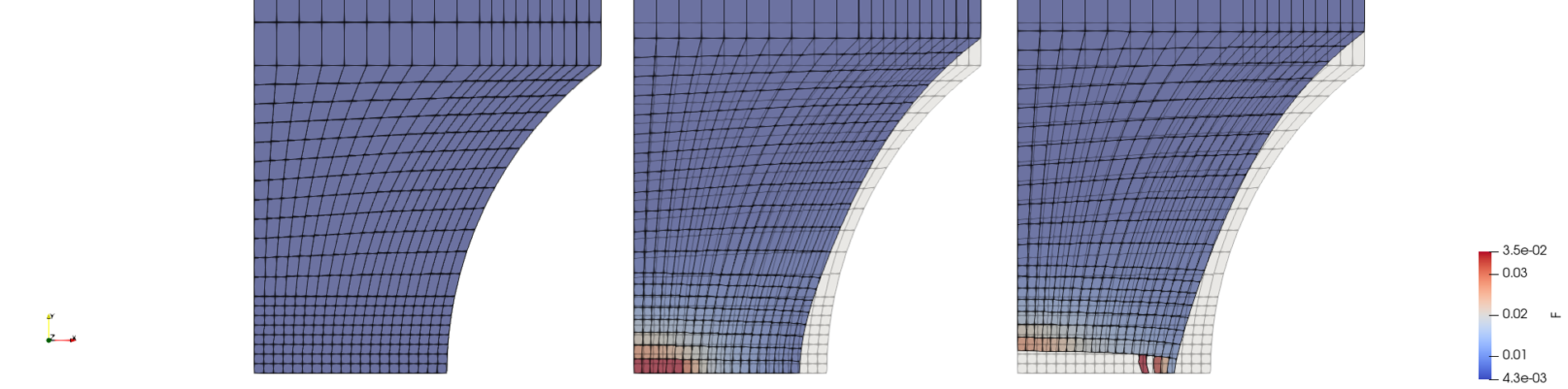
Moreover, the evolution of the porosity was monitored during the simulation to observe the failure of elements that reached the critical porosity value. This could be seen on Figure 5 where the notch is pictured before the testing (left image), during the testing (middle image), and at failure (right image).

6.2 Charpy test simulations

The GTN model is used to perform a simulation of a Charpy test. The parameters of the model are taken from [14] and correspond to the mechanical behavior of a Reactor Pressure Vessel steel at \(300^{\circ}\)C. The corresponding MFront implementation of the constitutive equations is:

Material’s Behavior

@DSL Implicit;
@Behaviour GTN;
@UMATUseTimeSubStepping true;
@UMATMaximumSubStepping 100;
@ModellingHypotheses{".+"};
@StrainMeasure Hencky;
@Algorithm NewtonRaphson;
@Epsilon 1.e-12;
@Theta 1;
@Brick StandardElastoViscoPlasticity{
 stress_potential : "Hooke" {young_modulus : 210e3, poisson_ratio : 0.3},
 inelastic_flow : "Norton" {
   criterion : "GursonTvergaardNeedleman1982" {
     f_c : 0.001,
     f_r : 0.33,
     q_1 : 1.5,
     q_2 : 1,
     q_3 : 2.25
   },
   n : 1.15,
   K : 0.185,
   A : 1,
   isotropic_hardening : "Linear" {R0 : 421.5},
   isotropic_hardening : "Voce" {R0 : 0, Rinf : 125, b : 59.6},
   isotropic_hardening : "Voce" {R0 : 0, Rinf : 472, b : 1.72}
 },
 porosity_evolution : {
   nucleation_model : "PowerLaw (strain)" {
      fn : 0.038, en : 0.5, m : 0., fmax : 0.023}
 }
}

Simulations are performed with Cast3M finite element code, using second-order reduced-integration elements (user-modified CU20 elements). Contact is modelled between the specimen and the striker and anvils accounting for friction (\(\mu = 0.1\)). Only one fourth of the system is modelled due to symmetries. The initial porosity is equal to 0.0175%. The displacement of the striker is imposed with a velocity of \(5\mathrm{m.s^{-1}}\). The time-step is adjusted with a target on the maximal increase of local porosity of 0.1% (see Appendix F). Element deletion is activated when at least half of the Gauss points are broken. In addition, Gauss points where the cumulated plastic strain is higher than \(200\%\) are considered as broken.

The evolution of the force as a function of the imposed displacement of the stricker is shown in Figure 6 where the decrease is related to the propagation of the crack. Figure 6 shows also the cumulated plastic strain field on the deformed configuration.

7 Conclusions

This report has described the extension of the StandardElastoViscoPlasticity brick to porous plasticity. Various new stress criteria and nucleation models have been implemented and can be used “out of the box.” A particular attention has been paid to ease the addition of new porous stress criteria and nucleation models.

An original staggered algorithm has been proposed and tested on ductile fracture simulations of notched specimens and Charpy tests. Note that the standard implicit scheme can still be chosen.

8 Appendix

8.1 Determination of the stress criterion through a local scalar Newton algorithm

In many cases, the stress criterion \(\sigma_{\star}\) is an implicit function of the stress state of the form:

\[ S{\left(\sigma_{\star}, \underline{\sigma}, f\right)}=0 \qquad(19)\]

See Equations (1) and (2) for the case of the Gurson-Tvergaard-Needleman stress criterion and the Rousselier-Tanguy-Besson stress criterion respectively.

For a given stress state and porosity, Equation (19) may be solved by a scalar Newton algorithm.

The Newton algorithm is coupled with bisection whenever root-bracketting is possible, which considerably increase its robustness.

More precisely, if not given by the user, the algorithm tries to determines a interval \(\left[\sigma_{\star}^{\min{}};\sigma_{\star}^{\max{}}\right]\) such that:

\[ S{\left(\sigma_{\star}^{\min{}}\right)}\,S{\left(\sigma_{\star}^{\max{}}\right)}<0 \]

i.e. \(S{\left(\sigma_{\star}^{\min{}}\right)}\) and \(S{\left(\sigma_{\star}^{\max{}}\right)}\) have opposite signs. If such a pair is found, a simple bissection algorithm, whose convergence is guaranteed, may be used.

In practice, one checks if the new estimate given by the Newton algorithm lies in \(\left[\sigma_{\star}^{\min{}};\sigma_{\star}^{\max{}}\right]\). If this is the case, this new estimate is used to update the bounds of the interval.

This implementation handles properly IEEE754 exceptional cases (infinite numbers, NaN values), even if advanced compilers options are used (such as -ffast-math under gcc).

8.2 Derivatives of common nucleation law

• Chu-Needleman strain based [9]

\[ \begin{aligned} \dfrac{\partial A_n}{\partial \underline{\sigma}} &= \underline{0} \\ \dfrac{\partial A_n}{\partial p} &= -\dfrac{f_N}{s_N^2 \sqrt{2\pi}} {\left(\dfrac{p - \epsilon_N}{s_N} \right)} \exp{{\left(-\dfrac{1}{2} {\left(\dfrac{p - \epsilon_N}{s_N} \right)}^2 \right)} } \\ \dfrac{\partial A_n}{\partial f} &= 0 \\ \end{aligned} \]

• Chu-Needleman stress based [9]

\[\dfrac{\partial A_n}{\partial \underline{\sigma}} = -\dfrac{f_N}{s_N^2 \sqrt{2\pi}} {\left(\dfrac{\sigma_I - \sigma_N}{s_N} \right)} \exp{{\left(-\dfrac{1}{2} {\left(\dfrac{\sigma_I - \sigma_N}{s_N} \right)}^2 \right)} } e_I \otimes e_I \]

\[\dfrac{\partial A_n}{\partial p} = 0 \]

\[\dfrac{\partial A_n}{\partial f} = 0 \]

• Power-Law strain based

\[ \begin{aligned} \dfrac{\partial A_n}{\partial \underline{\sigma}} &= \underline{0} \\ \dfrac{\partial A_n}{\partial p} &= \dfrac{m f_N}{\epsilon_N} \left<\dfrac{p}{\epsilon_N} - 1 \right>^{m-1} \\ \dfrac{\partial A_n}{\partial f} &= 0 \\ \end{aligned} \]

• Power-Law stress based

\[\dfrac{\partial A_n}{\partial \underline{\sigma}} = \dfrac{m f_N}{\sigma_N} \left<\dfrac{\sigma_I}{\sigma_N} - 1 \right>^{m-1} e_I \otimes e_I \]

\[\dfrac{\partial A_n}{\partial p} = 0 \]

\[\dfrac{\partial A_n}{\partial f} = 0 \]

8.3 Derivatives of standard stress criteria

8.3.1 Derivatives of the Gurson-Tvergaard-Needleman stress criterion

As \(\sigma_{\star}\) is defined implicitly through \(S(\underline{\sigma},\sigma_{\star},f) =0\), the first and second order derivatives of the function S are required to compute the first and second order derivatives of \(\sigma_{\star}\):

\[ \begin{aligned} {\displaystyle \frac{\displaystyle \partial S}{\displaystyle \partial \sigma_{\star}}} &= -2 \dfrac{\sigma_{vM}^2}{\sigma_{\star}^3} - \dfrac{3 q_1 q_2 f_{\star} \sigma_m}{\sigma_{\star}^2}\sinh{{\left(\dfrac{3}{2} q_2 \dfrac{\sigma_m}{\sigma_{\star}}\right)}} \\ \dfrac{\partial S}{\partial {\underline{\sigma}}} &= 3 \dfrac{\underline{s}}{\sigma_{\star}^2} + \dfrac{q_1 q_2 f_{\star}}{\sigma_{\star}}\sinh{{\left(\dfrac{3}{2} q_2 \dfrac{\sigma_m}{\sigma_{\star}}\right)}} \underline{I} \\ {\displaystyle \frac{\displaystyle \partial S}{\displaystyle \partial f}} &= 2 q_1 \delta \cosh{{\left(\dfrac{3}{2} q_2 \dfrac{\sigma_m}{\sigma_{\star}}\right)}} - 2 q_3 \delta f_{\star}\\ \dfrac{\partial^2 S}{\partial \underline{\sigma}^2} &= \dfrac{2}{\sigma_{\star}^2} \: {\underline{\underline{\mathbf{M}}}} + \dfrac{ q_1 \: q_2^2 \: f_{\star}}{2 \sigma_{\star}^2} \cosh{{\left(\dfrac{3}{2} q_2 \dfrac{\sigma_m}{\sigma_{\star}}\right)}} \underline{I} \otimes \underline{I}\\ \dfrac{\partial^2 S}{\partial \underline{\sigma}\partial \sigma_{\star}} &= - \dfrac{6 \underline{s}}{\sigma_{\star}^3} - \dfrac{ q_1 \: q_2 \: f_{\star}}{\sigma_{\star}^2} \sinh{{\left(\dfrac{3}{2} q_2 \dfrac{\sigma_m}{\sigma_{\star}}\right)}} \underline{I} - \dfrac{3 \: q_1 \: q_2^2 \: f_{\star} \: \sigma_m}{2 \: \sigma_{\star}^3} \cosh{{\left(\dfrac{3}{2} q_2 \dfrac{\sigma_m}{\sigma_{\star}}\right)}} \underline{I}\\ \dfrac{\partial^2 S}{\partial \underline{\sigma}\partial f} &= \dfrac{q_1 \: q_2 \: \delta}{\sigma_{\star}} \sinh{{\left(\dfrac{3}{2} q_2 \dfrac{\sigma_m}{\sigma_{\star}}\right)}} \underline{I} \\ \dfrac{\partial^2 S}{\partial \sigma_{\star}\partial f} &= - \dfrac{3 \: q_1 \: q_2 \: \delta \: \sigma_m}{\sigma_{\star}^2} \sinh{{\left(\dfrac{3}{2} q_2 \dfrac{\sigma_m}{\sigma_{\star}}\right)}} \\ \dfrac{\partial^2 S}{\partial \sigma_{\star}^2} &= 6 \dfrac{\sigma_{vM}^2}{\sigma_{\star}^4} + \dfrac{6 q_1 q_2 f_{\star} \sigma_m}{\sigma_{\star}^3}\sinh{{\left(\dfrac{3}{2} q_2 \dfrac{\sigma_m}{\sigma_{\star}}\right)}} + \dfrac{9 q_1 q_2^2 f_{\star} \sigma_m^2}{2\sigma_{\star}^4}\cosh{{\left(\dfrac{3}{2} q_2 \dfrac{\sigma_m}{\sigma_{\star}}\right)}} \end{aligned} \]

The first and second order derivatives of \(\sigma_{\star}\) are:

\[{\displaystyle \frac{\displaystyle \partial \sigma_{\star}}{\displaystyle \partial \underline{\sigma}}} = -{\left({\displaystyle \frac{\displaystyle \partial S}{\displaystyle \partial \sigma_{\star}}} \right)}^{-1} \dfrac{\partial S}{\partial {\underline{\sigma}}}\]

\[{\displaystyle \frac{\displaystyle \partial \sigma_{\star}}{\displaystyle \partial f}} = -{\left({\displaystyle \frac{\displaystyle \partial S}{\displaystyle \partial \sigma_{\star}}} \right)}^{-1} \dfrac{\partial S}{\partial {f}}\]

\[ \dfrac{\partial^2 \sigma_{\star}}{\partial \underline{\sigma}^2} = - \bigg({\displaystyle \frac{\displaystyle \partial S}{\displaystyle \partial \sigma_{\star}}} \bigg)^{-1} \bigg(\dfrac{\partial^2 S}{\partial \underline{\sigma}^2} + \dfrac{\partial^2 S}{\partial \underline{\sigma}\partial \sigma_{\star}} \otimes {\displaystyle \frac{\displaystyle \partial \sigma_{\star}}{\displaystyle \partial \underline{\sigma}}} \bigg) + \bigg({\displaystyle \frac{\displaystyle \partial S}{\displaystyle \partial \sigma_{\star}}} \bigg)^{-2} \bigg({\displaystyle \frac{\displaystyle \partial S}{\displaystyle \partial \underline{\sigma}}} \bigg) \otimes \bigg(\dfrac{\partial^2 S}{\partial \underline{\sigma}\partial \sigma_{\star}} + \dfrac{\partial^2 S}{ \partial \sigma_{\star}^2} {\displaystyle \frac{\displaystyle \partial \sigma_{\star}}{\displaystyle \partial \underline{\sigma}}} \bigg) \]

\[\dfrac{\partial^2 \sigma_{\star}}{\partial \underline{\sigma}\partial f} = - \bigg(\dfrac{\partial S}{\partial \sigma_{\star}} \bigg)^{-1} \bigg(\dfrac{\partial^2 S}{\partial \underline{\sigma}\partial f} + \dfrac{\partial^2 S}{\partial f \partial \sigma_{\star}} {\displaystyle \frac{\displaystyle \partial \sigma_{\star}}{\displaystyle \partial \underline{\sigma}}} \bigg) + \bigg(\dfrac{\partial S}{\partial \sigma_{\star}} \bigg)^{-2} \bigg(\dfrac{\partial^2 S}{\partial \underline{\sigma}\partial \sigma_{\star}} + \dfrac{\partial^2 S}{ \partial \sigma_{\star}^2} {\displaystyle \frac{\displaystyle \partial \sigma_{\star}}{\displaystyle \partial \underline{\sigma}}} \bigg) \bigg({\displaystyle \frac{\displaystyle \partial S}{\displaystyle \partial f}} \bigg) \]

8.3.2 Derivatives of Rousselier-Tanguy-Besson stress criterion

The first and second order derivatives of \(\sigma_{\star}\) are computed using \(S(\underline{\sigma},\sigma_{\star},f) =0\), which requires the first and second order derivatives of the function S:

\[ \begin{aligned} {\displaystyle \frac{\displaystyle \partial S}{\displaystyle \partial \sigma_{\star}}} &= -\dfrac{\sigma_{vM}}{(1- f )\sigma_{\star}^2} - f D_R q_R \dfrac{\sigma_{m}}{(1- f )\sigma_{\star}^2} \exp{{\left(\dfrac{3}{2} q_R \dfrac{\sigma_m}{(1 - f )\sigma_{\star}} \right)}}\\ \dfrac{\partial S}{\partial {\underline{\sigma}}} &= \dfrac{3}{2}\dfrac{\underline{s}}{(1- f ) \sigma_{vM} \sigma_{\star}} + \dfrac{f D_R q_R}{3} \dfrac{\underline{I}}{(1- f )\sigma_{\star}} \exp{{\left(\dfrac{3}{2} q_R \dfrac{\sigma_m}{(1 - f )\sigma_{\star}} \right)}} \\ {\displaystyle \frac{\displaystyle \partial S}{\displaystyle \partial f}} &= \dfrac{\sigma_{vM}}{\sigma_{\star}(1-f)^2} + \dfrac{2}{3} D_R \exp{{\left(\dfrac{3}{2} q_R \dfrac{\sigma_m}{(1 - f )\sigma_{\star}} \right)}} {\left(1 + \dfrac{3 f q_R \sigma_m}{2 \sigma_{\star}(1-f)^2} \right)} \\ \dfrac{\partial^2 S}{\partial \underline{\sigma}^2} &= \dfrac{3}{2(1-f)\sigma_{\star}\sigma_{vM} } {\left( \dfrac{2}{3} {\underline{\underline{\mathbf{M}}}} - \dfrac{3}{2} \dfrac{\underline{s}}{\sigma_{vM}} \otimes \dfrac{\underline{s}}{\sigma_{vM}} \right)} + \dfrac{f D_R q_R^2 }{6 (1-f)^2 \sigma_{\star}^2} \underline{I} \otimes \underline{I} \exp{{\left(\dfrac{3}{2} q_R \dfrac{\sigma_m}{(1 - f )\sigma_{\star}} \right)}}\\ \dfrac{\partial^2 S}{\partial \underline{\sigma}\partial \sigma_{\star}} &= - \dfrac{3 \underline{s}}{2 (1-f) \sigma_{vM} \sigma_{\star}^2 } - {\left(1 + \dfrac{3 q_R \sigma_m}{2 (1- f) \sigma_{\star}}\right)} \dfrac{f D_R q_R}{3 (1-f) \sigma_{\star}^2} \exp{{\left(\dfrac{3}{2} q_R \dfrac{\sigma_m}{(1 - f )\sigma_{\star}} \right)}} \underline{I}\\ \dfrac{\partial^2 S}{\partial \underline{\sigma}\partial f} &= \dfrac{3 \underline{s}}{2 (1-f)^2 \sigma_{vM} \sigma_{\star}} + {\left(1 + \dfrac{3 q_R \sigma_m}{2 (1 - f) \sigma_{\star}} + \dfrac{1-f}{f}\right)} \dfrac{f D_R q_R}{3 (1-f)^2 \sigma_{\star}} \exp{{\left(\dfrac{3}{2} q_R \dfrac{\sigma_m}{(1 - f )\sigma_{\star}} \right)}} \underline{I} \\ \dfrac{\partial^2 S}{\partial \sigma_{\star}\partial f} &= -\dfrac{\sigma_{vM} }{(1-f)^2 \sigma_{\star}^2 } - {\left(1 + \dfrac{3 q_R \sigma_m}{2 (1 - f) \sigma_{\star}} + \dfrac{1-f}{f}\right)} \dfrac{f D_R q_R \sigma_m}{ (1-f)^2 \sigma_{\star}^2} \exp{{\left(\dfrac{3}{2} q_R \dfrac{\sigma_m}{(1 - f )\sigma_{\star}} \right)}} \\ \dfrac{\partial^2 S}{\partial \sigma_{\star}^2} &= \dfrac{2\sigma_{vM}}{(1-f)\sigma_{\star}^3} + {\left(1 + \dfrac{3 q_R \sigma_m}{4 (1-f) \sigma_{\star}}\right)} \dfrac{2fD_Rq_R \sigma_m}{(1-f)\sigma_{\star}^3} \exp{{\left(\dfrac{3}{2} q_R \dfrac{\sigma_m}{(1 - f )\sigma_{\star}} \right)}} \end{aligned} \]

The first and second order derivatives of \(\sigma_{\star}\) are:

\[{\displaystyle \frac{\displaystyle \partial \sigma_{\star}}{\displaystyle \partial \underline{\sigma}}} = -{\left({\displaystyle \frac{\displaystyle \partial S}{\displaystyle \partial \sigma_{\star}}} \right)}^{-1} \dfrac{\partial S}{\partial {\underline{\sigma}}}\]

\[{\displaystyle \frac{\displaystyle \partial \sigma_{\star}}{\displaystyle \partial f}} = -{\left({\displaystyle \frac{\displaystyle \partial S}{\displaystyle \partial \sigma_{\star}}} \right)}^{-1} \dfrac{\partial S}{\partial {f}}\]

\[ \dfrac{\partial^2 \sigma_{\star}}{\partial \underline{\sigma}^2} = - \bigg({\displaystyle \frac{\displaystyle \partial S}{\displaystyle \partial \sigma_{\star}}} \bigg)^{-1} \bigg(\dfrac{\partial^2 S}{\partial \underline{\sigma}^2} + \dfrac{\partial^2 S}{\partial \underline{\sigma}\partial \sigma_{\star}} \otimes {\displaystyle \frac{\displaystyle \partial \sigma_{\star}}{\displaystyle \partial \underline{\sigma}}} \bigg) + \bigg({\displaystyle \frac{\displaystyle \partial S}{\displaystyle \partial \sigma_{\star}}} \bigg)^{-2} \bigg({\displaystyle \frac{\displaystyle \partial S}{\displaystyle \partial \underline{\sigma}}} \bigg) \otimes \bigg(\dfrac{\partial^2 S}{\partial \underline{\sigma}\partial \sigma_{\star}} + \dfrac{\partial^2 S}{ \partial \sigma_{\star}^2} {\displaystyle \frac{\displaystyle \partial \sigma_{\star}}{\displaystyle \partial \underline{\sigma}}} \bigg) \]

\[\dfrac{\partial^2 \sigma_{\star}}{\partial \underline{\sigma}\partial f} = - \bigg(\dfrac{\partial S}{\partial \sigma_{\star}} \bigg)^{-1} \bigg(\dfrac{\partial^2 S}{\partial \underline{\sigma}\partial f} + \dfrac{\partial^2 S}{\partial f \partial \sigma_{\star}} {\displaystyle \frac{\displaystyle \partial \sigma_{\star}}{\displaystyle \partial \underline{\sigma}}} \bigg) + \bigg(\dfrac{\partial S}{\partial \sigma_{\star}} \bigg)^{-2} \bigg(\dfrac{\partial^2 S}{\partial \underline{\sigma}\partial \sigma_{\star}} + \dfrac{\partial^2 S}{ \partial \sigma_{\star}^2} {\displaystyle \frac{\displaystyle \partial \sigma_{\star}}{\displaystyle \partial \underline{\sigma}}} \bigg) \bigg({\displaystyle \frac{\displaystyle \partial S}{\displaystyle \partial f}} \bigg) \]

8.4 Regularization of the effective porosity

The Gurson-Tvergaard-Needleman stress criterion models the void coalescence by the effective porosity calculated as shown above. The transition from the pre-coalescence to the coalescence phase might cause numerical problems if the \(\delta\) parameter is high enough. This is due to the inflection point in the bilinear function describing \(f_{\star}\) as a function of \(f\). Therefore, the first derivative of the effective porosity with respect to the porosity (\(\dfrac{\partial f_{\star}}{\partial f}\)) undergoes a sudden jump that disturbs the Newton-Raphson algorithm.

A solution is proposed to avoid that derivative jump at the inflection point : to replace the bilinear function of \(f_{\star}\) by a polynominal function of 5th degree. Therefore, \(f_{\star}\) is defined such that :

\[ f_{\star} = \left\{ \begin{array}{ll} \delta f & \mbox{if } f < (f_c - \epsilon) \\ \delta (a^5 f + b^4 f + c^3 f + d^2 f + e f + g) & \mbox{if } (f_c - \epsilon) \leq f \leq (f_c + \epsilon) \\ f_c + \delta (f - f_c) & \mbox{otherwise} \end{array} \right. \]

and :

\[ \delta = \left\{ \begin{array}{ll} 1 & \mbox{if } f \leq (f_c + \epsilon) \\ \dfrac{\dfrac{1}{q_1} - f_c }{f_r - f_c} & \mbox{otherwise} \end{array} \right. \]

where \(\epsilon\) is the linearization coefficient that allows to have a smooth transition on the \(\partial f_{\star}\) as function of \(f\). A big \(\epsilon\) value will allow a higher contribution of the polynominal function and thus, smoother numerical convergence.

For numerical efficiency reasons, the polynominal function was implemented using the Horner method to be :

\[ f (f ( f (f (a f + b) + c) + d) + e) + g\]

8.5 On the use of porous constitutive equations with Cast3M

The staggered approach improves robustness of the numerical integration of the porous constitutive equations, especially if sub-stepping is allowed. However, integration may still fail due to too severe input parameters. As integration failure is not handled in the finite element code Cast3M, additional stategies are required at the structural scale to avoid such problems. An efficient stategy is to adjust the time-step based on the maximal increase of porosity such as: \[ \Delta t_{i+1} = \min{\left( \frac{\Delta f_{max}}{\Delta f_{i}} \Delta t_i , \Delta t_{ref} \right)} \] This equation is implemented in two steps. First, the following code is added to the PERSO1 user procedure to compute the maximal increase of porosity at the last time-step on unbroken Gauss points.

'SI'( ('DIME' TAB1.DEPLACEMENTS) > 1);

TMP =  TAB1.'F_PREC';
TMP2 = 'EXCO' TAB1.ESTIMATION.VARIABLES_INTERNES 'F' 'SCAL';
TMP3 = 'EXCO' TAB1.ESTIMATION.VARIABLES_INTERNES 'BROK' 'SCAL';

TMPA = TMP*(1 '-' TMP3);
TMP2A = TMP2*(1 '-' TMP3);

DF = 'ABS' (('MAXIMUM' TMPA) '-' ('MAXIMUM' TMP2A));

TAB1.'F_PREC' = TMP2;

'SINON';

DF = 0;

'FINSI';

TAB1.WTABLE.'DF' = DF;
TAB1.WTABLE.'DFMAX' = TAB1.'DFMAX';

Then, the PASAPAS procedure is modified according to:

'SI' WTAB.'PAS_AJUSTE';
   DTV = DT_AVANT;
   DF = WTAB.'DF';
   DFMAX = WTAB.'DFMAX';
   DDF = DF '/' DFMAX;
   'SI' ('EXISTE' WTAB ISOUSPAS);
      ISP = WTAB.ISOUSPAS;
   'SINON';
      ISP = 0;
   'FINSI';
   'SI' WTAB.'CONV';
      'SI' ((DDF > 1));
         DTV = DTV '/' DDF;
      'FINSI';
      'SI' ((DDF < 1) 'ET' (ISP 'EGA' 0));
         'SI' IREREDU;
            'SI' (DDF > 0.5);
               DTV = DTV '/' DDF;
            'SINON';
               DTV = DTV '/' 0.5;
            'FINSI';   
         'FINSI';
      'FINSI';
      DT_AVANT = DTV;
      IREREDU = VRAI;
      'SINON';
         DTV=0.0000000001D0* DT_AVANT;
         DT_AVANT= DT_AVANT /2.;
         IREREDU=FAUX;
      'FINSI';
      TTI = DTV* 1.0000000001 + TEMP0;
      'SI' ( TTI '<EG' TIV );
         TI=TTI;
         PASFINAL=0;
      'FINSI';
   'FINSI';

The time-step is adjusted in order to target a maximal local increase of porosity lower or equal to an user-defined value DFMAX. In addition, increasing the time-step is allowed only if the convergence of the last time-step was achieved without sub-stepping (through CONVERGENCE_FORCEE).

In addition, global convergence may be difficult to achieve in cases where heavily-distorted elements are present. Element-deletion is detailed below, but a slight modification of the UNPAS procedure can be made to lower the precision of the computation when sub-steps are done, allowing to avoid premature end of the calculation:

*Nombre maximum de sous-pas atteint? si oui, arret de pasapas
WTAB.'ISOUSPAS' = WTAB.'ISOUSPAS' + 1;
ZPREC = ZPREC * 2;
ZPRECM = ZPRECM * 2;

Finally, an example of element deletion that can be added to the PERSO1 procedure can be added, based on the number of broken Gauss points and cumulated plastic strain:

MO1 = TAB1.WTABLE.'MO_TOT';
MA1 = TAB1.WTABLE.'MA_TOT';
MAIL1 = 'EXTRAIRE' MO1 'MAIL';
TMP1 = 'EXCO' (TAB1.ESTIMATION.VARIABLES_INTERNES) 'BROK' 'SCAL';
TMP2 = 'EXCO' (TAB1.ESTIMATION.VARIABLES_INTERNES) 'P' 'SCAL'; 
TMP2 = TMP2 'MASQ' SUPE (TAB1.'BROKEN_STRAIN');

TMP1 = (TMP1 + TMP2) MASQ SUPE 0.;
TMP1 = 'CHANGER' GRAVITE MO1 TMP1 'STRESSES';
TMP1 = TMP1 'MASQUE' 'EGSU' 0.5;

MEBR = TMP1 'ELEM' SUPE 0.;
MESO = 'DIFF' MAIL1 MEBR;
NBRO = 'NBEL' MEBR;

TAB1.'DBRO' = TAB1.'DBRO' '+' NBRO;
TAB1.'NBRO' = TAB1.'NBRO' '+' NBRO;

'SI' ('>' NBRO 0);

MO2 = 'REDU' MO1 MESO;
TAB1.WTABLE.'MO_TOT' = MO2;
TAB1.WTABLE.'MO_TOTAL' = MO2;
TAB1.WTABLE.'MOD_MEC' = MO2;

'FINSI';

8.6 Options of the porosity_evolution section

This appendix is dedicated to the description of the various options that can be declared in the porosity_evolution section inside the declaration of the StandardElastoViscoPlasticity brick:

• save_individual_porosity_increase: a boolean value stating if the each contribution to the porosity increase must be stored in a dedicated state variable or auxiliary state variable. By default, this option is set to false.
• elastic_contribution: a boolean value stating if the elastic contribution to the porosity growth must be taken into account. By default, this option is set to false.
• nucleation_model: this option introduces a new nucleation model.
• algorithm: a string value which allow the selection of the resolution algorithm. Valid values are:
  • standard implicit scheme
  • standard_implicit_scheme
  • StandardImplicitScheme
  • staggered scheme
  • staggered_scheme
  • StaggeredScheme The algorithm may have suboptions, as described in Section
• safety_factor_for_the_upper_bound_of_the_porosity: this option allows setting floatting-point value, denoted \(\alpha\), which is used to determine the maximum value of the porosity at the middle of the time step as \(\alpha\,f_{r}\), where \(f_{r}\) is the upper bound of the porosity. The upper bound of the porosity is equal the minimum of the coalescence porosity of all selected stress criteria or is equal to \(1\) if no stress criterion declares a coalescence porosity. By default, the value of this option is \(0.985\).
• safety_factor_for_the_upper_bound_of_the_porosity_for_fracture_detection: this option allows setting floatting-point value, denoted \(\alpha\), which is used by the staggered algorithm to detect the failure of the material. The failure is detected when the porosity converges to a value greater than \(\alpha\,f_{r}\) where \(f_{r}\) is the upper bound of the porosity. By default, the value of this option is \(0.984\).

8.6.1 Suboptions of the algorithm option

When a staggered scheme is used, two numerical parameters can be specified:

• convergence_criterion: the value of the convergence criterion of the staggered algorithm. The staggered scheme stops when the difference between two estimates of the porosity is lower than this value. The default value is \(1.e-10\).
• maximum_number_of_iterations: the maximum number of iterations allows for the staggered scheme. The default value is \(100\).

Here is a simple example on how to specify those numerical parameters:

  porosity_evolution: {
    algorithm : "staggered_scheme" {
      convergence_criterion: 1.e-9,
      maximum_number_of_iterations: 200
    }
  }

References