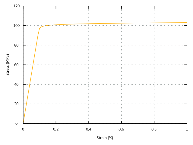
In fracture mechanics, it is classical to replace the plastic behaviour by an equivalent non linear elastic behaviour.
This document describes the implementation of non linear elastic
behaviour of the Ramberg-Osgood type using the Default
domain specific language of MFront.
The full implementation is available here.
Note
This implementation is compatible with
MFront-3.3and uses unicode characters (see this page for details).
The behaviour is based on the following relationship between the strain \(\underline{\varepsilon}^{\mathrm{to}}\) and the stress \(\underline{\sigma}\):
\[ \underline{\varepsilon}^{\mathrm{to}}= {{\displaystyle \frac{\displaystyle 1}{\displaystyle 3\,K}}}\,{\mathrm{tr}{\left(\underline{\sigma}\right)}}\,\underline{I}+ {{\displaystyle \frac{\displaystyle \sigma_{\mathrm{eq}}}{\displaystyle 3\,\mu}}}\,\underline{n}+ \alpha\,{\left({{\displaystyle \frac{\displaystyle \sigma_{\mathrm{eq}}}{\displaystyle \sigma_{0}}}}\right)}^{n}\,\underline{n} \qquad{(1)}\]
where:
Knowing the strain \(\underline{\varepsilon}^{\mathrm{to}}\), integration of the behaviour, which boils down to the computation of the stress \(\underline{\sigma}\), requires the inversion of Equation (1).
The projection of this equation on the volumetric axis yields:
\[ {\mathrm{tr}{\left(\underline{\sigma}\right)}}=K\,{\mathrm{tr}{\left(\underline{\varepsilon}^{\mathrm{to}}\right)}} \]
Taking the deviatoric part of Equation (1) yields:
\[ \underline{s}^{e}= {\left({{\displaystyle \frac{\displaystyle \sigma_{\mathrm{eq}}}{\displaystyle 3\,\mu}}}+ \alpha\,{\left({{\displaystyle \frac{\displaystyle \sigma_{\mathrm{eq}}}{\displaystyle \sigma_{0}}}}\right)}^{n}\right)}\,\underline{n} = f{\left(\sigma_{\mathrm{eq}}\right)}\,\underline{n} \qquad{(2)}\]
Contracting each side of his equations with itself leads to:
\[ \underline{s}^{e}\,\colon\,\underline{s}^{e} = f^{2}{\left(\sigma_{\mathrm{eq}}\right)}\, \underline{n}\,\colon\,\underline{n} = {{\displaystyle \frac{\displaystyle 3}{\displaystyle 2}}}\,f^{2}{\left(\sigma_{\mathrm{eq}}\right)} \]
where we used the classical result: \(\underline{n}\,\colon\,\underline{n}={{\displaystyle \frac{\displaystyle 3}{\displaystyle 2}}}\).
Finally, \(\sigma_{\mathrm{eq}}\) satisfies:
\[ f{\left(\sigma_{\mathrm{eq}}\right)}=\varepsilon_{\mathrm{eq}} \qquad{(3)}\]
with \(\varepsilon_{\mathrm{eq}}=\sqrt{{{\displaystyle \frac{\displaystyle 2}{\displaystyle 3}}}\,\underline{s}^{e}\,\colon\,\underline{s}^{e}}\).
The scalar Equation (3) allows resolving iteratively \(\sigma_{\mathrm{eq}}\) using a standard Newton-Raphson algorithm. Let \(\sigma_{\mathrm{eq}}^{(i)}\) be the current estimate of \(\sigma_{\mathrm{eq}}\), the next estimate is given by:
\[ \sigma_{\mathrm{eq}}^{(i+1)}=\sigma_{\mathrm{eq}}^{(i)}-{{\displaystyle \frac{\displaystyle f{\left(\sigma_{\mathrm{eq}}^{(i)}\right)}}{\displaystyle {\displaystyle \frac{\displaystyle \mathrm{d} f}{\displaystyle \mathrm{d} \sigma_{\mathrm{eq}}}}{\left(\sigma_{\mathrm{eq}}^{(i)}\right)}}}} \]
The initial estimation is choosen as follows:
\[ \sigma_{\mathrm{eq}}^{(0)}=\sigma_{0}\,\sqrt[n]{{{\displaystyle \frac{\displaystyle \varepsilon_{\mathrm{eq}}}{\displaystyle \alpha}}}} \]
Once \(\sigma_{\mathrm{eq}}\) is known, Equations (2) and (3) allow computing the normal \(\underline{n}\):
\[ \underline{n}= {{\displaystyle \frac{\displaystyle 1}{\displaystyle f{\left(\sigma_{\mathrm{eq}}\right)}}}}\,\underline{s}^{e}= {{\displaystyle \frac{\displaystyle 1}{\displaystyle \varepsilon_{\mathrm{eq}}}}}\,\underline{s}^{e} \]
The following relation allows computing the stress:
\[ \underline{\sigma} =K\,{\mathrm{tr}{\left(\underline{\varepsilon}^{\mathrm{to}}\right)}}\,\underline{I}+\underline{s} =K\,{\mathrm{tr}{\left(\underline{\varepsilon}^{\mathrm{to}}\right)}}\,\underline{I}+{{\displaystyle \frac{\displaystyle 2\,\sigma_{\mathrm{eq}}}{\displaystyle 3}}}\underline{n} =K\,{\mathrm{tr}{\left(\underline{\varepsilon}^{\mathrm{to}}\right)}}\,\underline{I}+{{\displaystyle \frac{\displaystyle 2\,\sigma_{\mathrm{eq}}}{\displaystyle 3\,\varepsilon_{\mathrm{eq}}}}}\,\underline{s}^{e} \]
Finally: \[ \underline{\sigma}=K\,{\mathrm{tr}{\left(\underline{\varepsilon}^{\mathrm{to}}\right)}}\,\underline{I}+\sigma_{\mathrm{eq}}\,\underline{n}^{e} \qquad{(4)}\] with \(\underline{n}^{e}={{\displaystyle \frac{\displaystyle 2}{\displaystyle 3\,\varepsilon_{\mathrm{eq}}}}}\,\underline{s}^{e}\).
The following relations will be useful: \[ \begin{aligned} {\displaystyle \frac{\displaystyle \mathrm{d} \varepsilon_{\mathrm{eq}}}{\displaystyle \mathrm{d} \underline{\varepsilon}^{\mathrm{to}}}}&=\underline{n}^{e}\\ {\displaystyle \frac{\displaystyle \mathrm{d} \underline{n}^{e}}{\displaystyle \mathrm{d} \underline{\varepsilon}^{\mathrm{to}}}}&= {{\displaystyle \frac{\displaystyle 1}{\displaystyle \varepsilon_{\mathrm{eq}}}}}{\left({{\displaystyle \frac{\displaystyle 2}{\displaystyle 3}}}\,\underline{\underline{\mathbf{P}}}-\underline{n}^{e}\,\otimes\,\underline{n}^{e}\right)}\\ \end{aligned} \] with \(\underline{\underline{\mathbf{P}}}=\underline{\underline{\mathbf{I}}}-{{\displaystyle \frac{\displaystyle 1}{\displaystyle 3}}}\,\underline{I}\,\otimes\,\underline{I}\)
Equation (4) allows computing the tangent operator as follows:
\[ {\displaystyle \frac{\displaystyle \mathrm{d} \underline{\sigma}}{\displaystyle \mathrm{d} \underline{\varepsilon}^{\mathrm{to}}}}= K\,\underline{I}\,\otimes\,\underline{I}+ {\displaystyle \frac{\displaystyle \mathrm{d} \sigma_{\mathrm{eq}}}{\displaystyle \mathrm{d} \varepsilon_{\mathrm{eq}}}}\,\underline{n}^{e}\,\otimes\,\underline{n}^{e}+ \sigma_{\mathrm{eq}}\,{\displaystyle \frac{\displaystyle \mathrm{d} \underline{n}^{e}}{\displaystyle \mathrm{d} \underline{\varepsilon}^{\mathrm{to}}}} \qquad{(5)}\]
\({\displaystyle \frac{\displaystyle \mathrm{d} \sigma_{\mathrm{eq}}}{\displaystyle \mathrm{d} \varepsilon_{\mathrm{eq}}}}\) is obtained by derivation of Equation (3) as follows:
\[ f{\left(\sigma_{\mathrm{eq}}{\left(\varepsilon_{\mathrm{eq}}\right)}\right)}=\varepsilon_{\mathrm{eq}}\Rightarrow {\displaystyle \frac{\displaystyle \mathrm{d} \sigma_{\mathrm{eq}}}{\displaystyle \mathrm{d} \varepsilon_{\mathrm{eq}}}}={{\displaystyle \frac{\displaystyle 1}{\displaystyle {\displaystyle \frac{\displaystyle \partial f}{\displaystyle \partial \sigma_{\mathrm{eq}}}}}}} \qquad{(6)}\]
While not mandatory (the @DSL keyword can be place
anywhere in the file), its is convenient to start the implementation by
declaring the domain specific language to be used. The
Default DSL, which does not set any particular integration
scheme, is the most appropriate here:
@DSL Default;The @Behaviour keyword is used to give the name of the
behaviour.
@Behaviour RambergOsgoodNonLinearElasticity;The following instructions give some information about the author, the date and some description of the behaviour.
@Author L. Gelebart/V. Duc Nguyen;
@Description {
  "Ramberg-Osgood model (non-(linear elastic formulation)"
  "Eps = S:Sig +β.σ_eq^n. N"
  "with:"
  " - N = (3/2) Sig_dev / σ_eq"
  " - σ_eq = rac((3/2)σ_dev:σ_dev))"
  " - β = α⋅σ₀/E"
}This behaviour is meant to be generic, which means that the specific characteristics of the material are to be given by the calling solver.
Here, we declare \(5\) material properties:
Cast3M solver.@MaterialProperty stress E;
E.setGlossaryName("YoungModulus");
@MaterialProperty real ν;
ν.setGlossaryName("PoissonRatio");
@MaterialProperty real n;
@MaterialProperty real α;
α.setEntryName("alpha");
@MaterialProperty stress σ₀;
σ₀.setGlossaryName("YieldStrength");Here, we use the subset of UTF-8 characters supported by
MFront (See this page for
details) to define the variables. Note that it is important to associate
so called external names to those variables using one of the
setEntryName and setGlossaryName methods: it
is highly recommended that the external names only contains
ASCII characters.
The following numerical parameter will be used as threshold to avoid division by zero.
//! Numerical threshold
@Parameter real e_ε = 1e-12;
e_ε.setEntryName("NumericalThreshold");The following local variables are used:
//! the shear modulus
@LocalVariable stress μ;
//! the bulk modulus
@LocalVariable stress K;
//! an helper variable
@LocalVariable real β;
//! von Mises equivalent stress
@LocalVariable stress σₑ;
/*!
 * derivative of the von Mises equivalent stress
 * with respect to the equivalent strain
 */
@LocalVariable stress ∂σₑ∕∂εₑ;
//! the equivalent strain
@LocalVariable strain εₑ;
//! inverse of the equivalent strain
@LocalVariable real iεₑ;
//! normal associated with the deviatoric part of the strain
@LocalVariable StrainStensor ne;
Local variables are available in each code blocks.
The initialisation of local variables is devoted to the
@InitLocalVariables.
@InitLocalVariables {
  μ = computeMu(E, ν);
  K = E / (3 ⋅ (1 - 2 ⋅ ν));
  β = α ⋅ σ₀ / E;
  σₑ = stress{};
  ∂σₑ∕∂εₑ = stress{};
}
Note that we use here the symbol ⋅ in place of
* as the multiplication sign. Both are equivalent.
The statement σₑ = stress{}; initializes σₑ
to a default value (which is 0).
The prediction operator can used by code_aster to
initialize the algorithm used to find the equilibrium. Here we only
implement an elastic prediction operator.
@PredictionOperator{
  const auto P = I₄ - (I₂ ⊗ I₂) / 3;
  Dt = K ⋅ (I₂ ⊗ I₂) + 2 ⋅ μ ⋅ P;
}
where:
I₄ is the fourth order identity tensor (of type
st2tost2, i.e. a fourth order tensor which transforms a
symmetric tensor to a a symmetric tensor).I₂ is the second order identity symmetric tensor⊗ is the tensorial product. It is equivalent to the
^ characters.The behaviour integration is @Integrator.
@Integrator{The integrator part is divided in three parts:
σₑ and its derivative ∂σₑ∕∂εₑ.The first part computes the strain at the end of the time step, its deviatoric part, the equivalent strain and the normal.
  const auto ε = εᵗᵒ + Δεᵗᵒ;
  const auto se = deviator(ε);
  εₑ = sqrt(2 ⋅ (se | se) / 3);
  iεₑ = 1 / max(εₑ, e_ε);
ne = 2 ⋅ se ⋅ (iεₑ / 3);The following code computes the von Mises stress and its derivative:
  if (εₑ < e_ε) {
    σₑ = 3 ⋅ μ ⋅ εₑ;
    ∂σₑ∕∂εₑ = 3 ⋅ μ;
  } else {
    const auto e_σ = E ⋅ e_ε;
    const auto i3μ = 1 / (3 ⋅ μ);
    auto f = real{};
    auto fidf = [&]() {
      const auto rσₑⁿ = pow(σₑ / σ₀, n);
      const auto iσₑ = 1 / max(e_σ, σₑ);
      f = σₑ ⋅ i3μ + β ⋅ rσₑⁿ - εₑ;
      ∂σₑ∕∂εₑ = 1 / max(i3μ + n ⋅ β ⋅ rσₑⁿ ⋅ iσₑ, i3μ ⋅ e_ε);
    };
    σₑ = σ₀ ⋅ pow(εₑ / β, 1 / n);
    auto iter = int{};
    fidf();
    while (abs(f) > e_ε) {
      fidf();
      σₑ -= f ⋅ ∂σₑ∕∂εₑ;
      if (++iter > 20) {
        throw(DivergenceException());
      }
    }
  }
If the equivalent strain is below the numerical threshold, a solution corresponding to an elastic behaviour is returned.
In the other case, a local Newton algorithm is used to determine
σₑ and ∂σₑ∕∂εₑ, as described by Section 2.1.
Except for the usage of a lambda function called ifdf, the
code is quite easy to read. A lambda function can be seen as a local
function which allows to factorise the code computing the residual and
its derivative. The syntax [&] means that the lambda
function of has access to all the variables of the surrounding scope by
references. Note that we used Equation (6) to identify \({{\displaystyle \frac{\displaystyle
1}{\displaystyle {\displaystyle \frac{\displaystyle \mathrm{d}
f}{\displaystyle \mathrm{d} \sigma_{\mathrm{eq}}}}}}}\) to
∂σₑ∕∂εₑ.
The computation of the stress is a direct translation of Equation (4):
σ = K ⋅ trace(ε) ⋅ I₂ + σₑ ⋅ ne;The @Integrator code block ends with a final curly
brace.
} // end of @IntegratorThe following block compute the tangent operator using Equation (5):
@TangentOperator{
  const auto P = I₄ - (I₂ ⊗ I₂) / 3;
  if ((smt == ELASTIC) || (smt == SECANTOPERATOR)) {
    Dt = K ⋅ (I₂ ⊗ I₂) + 2 ⋅ μ ⋅ P;
  } else {
    if (εₑ < e_ε) {
      Dt = K ⋅ (I₂ ⊗ I₂) + 2 ⋅ μ ⋅ P;
    } else {
      Dt = K ⋅ (I₂ ⊗ I₂) + ∂σₑ∕∂εₑ ⋅ (ne ⊗ ne) +
           σₑ ⋅ iεₑ ⋅ (2 ⋅ P / 3 - (ne ⊗ ne));
    }
  }
}