This document gives some insights on how a user may extend the StandardElastoViscoPlasticity brick by adding a new stress criterion coupled with porosity evolution.

The StandardElastoViscoPlasticity brick is fully described here.

Introducing a new porous stress criterion in the StandardElastoViscoPlasticity brick has two main steps:

• Extending the TFEL/Material library.
• Extending the TFELMFront library.

Note

This tutorial only covers isotropic stress criteria. Orthotropic stress criteria requires to take care of the orthotropic axes convention.

See the documentation of the @OrthotropicBehaviour keyword for details:

mfront --help-keyword=Implicit:@OrthotropicBehaviour

Those steps are illustrated by the implementation so-called hollow sphere criterion proposed by Michel and Suquet which describe the macroscopic viscoplasticty of a porous material by the following law (see [2]):

The viscoplastic strain rate is defined by:

\[ \underline{\dot{\varepsilon}}^{\mathrm{vp}}=\dot{\varepsilon}_{0}\,{\left({{\displaystyle \frac{\displaystyle \sigma_{\mathrm{eq}}^{MS}}{\displaystyle \sigma_{0}}}}\right)}^{E}\,\underline{n}^{MS} \]

where:

• \(\dot{\varepsilon}_{0}\) is a reference strain rate which shall be identified.
• \(\sigma_{0}\) is a reference stress used to normalise the stress.
• \(E\) is the Norton exponent.

The stress criterion \(\sigma_{\mathrm{eq}}^{MS}\) is defined by:

\[ \sigma_{\mathrm{eq}}^{MS}=\sqrt{{{\displaystyle \frac{\displaystyle 9}{\displaystyle 4}}}\,A{\left(f\right)}\,p^{2}+B{\left(f\right)}\,\sigma_{\mathrm{eq}}^{2}} \]

where:

• \(p\) is the hydrostatic pressure (\(p={{\displaystyle \frac{\displaystyle 1}{\displaystyle 3}}}{\mathrm{tr}{\left(\underline{\sigma}\right)}}\)).
• \(\sigma_{\mathrm{eq}}\) is the von Mises stress.
• \(A{\left(f\right)}={\left(n\,{\left(f^{-1/n}-1\right)}\right)}^{\frac{-2\,n}{n+1}}\)
• \(B{\left(f\right)}={\left(1+{{\displaystyle \frac{\displaystyle 2}{\displaystyle 3}}}\,f\right)}\,{\left(1-f\right)}^{\frac{-2\,n}{n+1}}\)
• \(n\) is the Norton exponent of the matrix

This flow is associated, to the flow direction is given by:

\[ \underline{n}^{MS}={\displaystyle \frac{\displaystyle \partial \sigma_{\mathrm{eq}}^{MS}}{\displaystyle \partial \underline{\sigma}}} \]

Implicit schemes

This document assumes that the reader has prior knowledge on how the integrate a behaviour using an implicit scheme with MFront.

Appropriate introductory materials are given in the gallery.

1 Extending the TFEL/Material library

1.1 Template files

We recommend that you use the following template files:

• PorousStressCriterionTemplate.hxx
• PorousStressCriterionTemplate.ixx
• PorousStressCriterionTest.mfront
• PorousStressCriterionTest_NumericalJacobian.mfront

The first file declares:

• A set of aliases
• A data structure holding the structure associated with the criterion.
• Three functions which allows the computation of:
  • The value of the stress criterion for the given stress state.
  • The value of the stress criterion and its first derivative for the given stress state.
  • The value of the stress criterion and its first and second derivatives for the given stress state.

The second file give a skeleton required to implement those three functions.

Implementing a new stress criterion boils down to the following steps:

1. Rename those file to explicitly indicate the name of the stress criterion.
2. Replace the following strings by the appropriate values as described below:

• __Author__
• __Date__
• __PorousStressCriterionName__
• __STRESS_CRITERION_NAME__

3. Implement the three previous functions
4. Test your implementation in MFront and MTest (or your favorite solver).

1.2 Creating a proper working directory for the example of the so-called hollow sphere criterion proposed by Michel and Suquet

In this paragraph, we detail Steps 1 and 2. for the case of the so-called hollow sphere criterion proposed by Michel and Suquet criterion (see [2]) which will be used as an illustrative example throughout this document. We describe all those steps in details and finally gives a shell script that automates the whole process for LiNuX users. When providing command line examples, we assume that the shell is bash.

The header files PorousStressCriterionTemplate.hxx and PorousStressCriterionTemplate.ixx are placed in a subdirectory called include/TFEL/Material and renamed respectively MichelAndSuquet1992HollowSphereTestStressCriterionTest.hxx and MichelAndSuquet1992HollowPorousStressCriterionTest.ixx.

The MFront template files must be copied in the working directory and renamed appropriatly.

This can be done by taping the following commands in the terminal (under LiNuX or Mac Os):

$ mkdir -p include/TFEL/Material
$ mkdir -p tests/test1
$ mv PorousStressCriterionTemplate.hxx \
     include/TFEL/Material/MichelAndSuquet1992HollowSphereTestStressCriterion.hxx
$ mv PorousStressCriterionTemplate.ixx \
     include/TFEL/Material/MichelAndSuquet1992HollowSphereTestStressCriterion.ixx
$ mv PorousStressCriterionTest.mfront \
     tests/test1/MichelAndSuquet1992HollowSphereTestViscoPlasticity.mfront
$ mv PorousStressCriterionTest_NumericalJacobian.mfront \
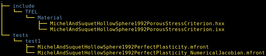
     tests/test1/MichelAndSuquet1992HollowSphereTestViscoPlasticity_NumericalJacobian.mfront

The working directory is thus organized as follows:

In all those files, we now replace

• __Author__ by Thomas Helfer, Jérémy Hure, Mohamed Shokeir
• __Date__ by 20/07/2020
• __StressCriterionName__ by MichelAndSuquet1992HollowSphereTest
• __STRESS_CRITERION_NAME__ by MICHEL_SUQUET_1992_HOLLOW_SPHERE_TEST

You may use your favourite text-editor to do this or use the following command (for LiNuX users) :

for f in $(find . -type f);                                                \
do sed -i                                                                  \
  -e 's|__Author__|Thomas Helfer, Jérémy Hure, Mohamed Shokeir|g;'         \
  -e 's|__Date__|24/03/2020|g;'                                            \
  -e 's|__StressCriterionName__|MichelAndSuquet1992HollowSphereTest|g;'                        \
  -e 's|__STRESS_CRITERION_NAME__|MICHEL_SUQUET_1992_HOLLOW_SPHERE_TEST|g' $f ; \
done

All those steps are summarized in the following script, which can be downloaded here.

In conclusion, a recommended for starting the development of the a new stress criterion is to download the previous script, modify appropriately the first lines to match your need and run it.

Note

At this stage, you shall already be able to verify that the provided MFront implementations barely compiles by typing in the tests/test1 directory:

mfront -I $(pwd)/../../include --obuild \
       --interface=generic        \
       MichelAndSuquet1992HollowSphereTestPerfectPlasticity.mfront

Note the -I $(pwd)/../../include flags which allows MFront to find the header files implementing the stress criterion (In bash, $(pwd) return the current directory).

1.3 Implementing the Michel and Suquet’ hollow sphere stress criterion

In this paragraph, we detail all the steps required to implement the Michel and Suquet’ hollow sphere stress criterion. In a new directory, we just follow the steps given by the previous paragraph:

wget https://thelfer.github.io/tfel/web/scripts/generate-porous.sh
chmod +x generate-porous.sh
./generate-porous.sh

1.3.1 Modifying the MichelAndSuquet1992HollowSphereTestStressCriterionParameters data structure

The MichelAndSuquet1992HollowSphereTestStressCriterionParameters data structure, declared in MichelAndSuquet1992HollowSphereTestStressCriterion.hxx, must contain the values of the Norton exponent of the matrix \(n\).

In the implementation, we will also need to define two small values:

• feps, which will be used to tell if the porosity is closed to its physical bounds, \(0\) and \(1\).
• feps2, which will be used to regularise the derivative \({\displaystyle \frac{\displaystyle \partial A}{\displaystyle \partial f}}\) as described below.

We modify it as follows:

template <typename StressStensor>
struct MichelAndSuquet1992HollowSphereTestStressCriterionParameters {
  //! a simple alias
  using real = MichelAndSuquet1992HollowSphereTestBaseType<StressStensor>;
  //! \brief \f$n\f$ is the Norton exponent of the matrix
  real n;
  //! \brief \f$feps\f$ is a small numerical parameter
  real feps = real(1e-14); 
  //! \brief \f$feps\f$ is a small numerical parameter
  real feps2 = real(1e-5); 
};  // end of struct MichelAndSuquet1992HollowSphereTestStressCriterionParameters

This is the only modification of the MichelAndSuquet1992HollowSphereTestStressCriterion.hxx file.

1.3.2 Include TFEL/Math/General/IEEE754.hxx header

The TFEL/Math/General/IEEE754.hxx header reimplements a set of standard functions which does not work as expected under gcc when the -ffast-math flag is used.

The header must be included at the top of the MichelAndSuquet1992HollowSphereTestStressCriterion.ixx file as follows:

#include "TFEL/Math/General/IEEE754.hxx"

1.3.3 Implementing the output stream operator for the MichelAndSuquet1992HollowSphereTestStressCriterionParameters data structure

The output stream operator must now be implemented in the MichelAndSuquet1992HollowSphereTestStressCriterion.ixx file:

template <typename StressStensor>
std::ostream &operator<<(std::ostream &os,
                         const MichelAndSuquet1992HollowSphereTestStressCriterionParameters<StressStensor> &p) {
  os << "{n: " << p.n << ", feps: " << p.feps << ", feps2: " << p.feps2 << "}";
  return os;
} // end of operator<<

This operator is useful when compiling MFront files in debug mode.

1.3.4 Implementing the computeMichelAndSuquet1992HollowSphereTestStress function

The computeMichelAndSuquet1992HollowSphereTestStress function is implemented in the MichelAndSuquet1992HollowSphereTestStressCriterion.ixx file.

The main difficulty is the computation of \(A{\left(f\right)}\) when the porosity ends toward \(0\). The limit is well defined, but the intermediate expression \(f^{-1/n}\) is undefined. To avoid this issue, we will use the following approximated expression:

\[ A_{\varepsilon}{\left(f\right)}={\left(n\,{\left(A_{0}{\left(f\right)}-1\right)}\right)}^{\frac{-2\,n}{n+1}}\quad\text{with}\quad A_{0}{\left(f\right)}= \left\{ \begin{aligned} {\left(n\,{\left({\left({{\displaystyle \frac{\displaystyle f+f_{\varepsilon}}{\displaystyle 2}}}\right)}^{-1/n}-1\right)}\right)}^{\frac{-2\,n}{n+1}}&\quad\text{if}\quad&f\leq f_{\varepsilon}\\ {\left(n\,{\left(f^{-1/n}-1\right)}\right)}^{\frac{-2\,n}{n+1}}&\quad\text{if}\quad&f> f_{\varepsilon} \end{aligned} \right. \]

With this expression, this implementation is straightforward:

template <typename StressStensor>
MichelAndSuquet1992HollowSphereTestStressType<StressStensor> computeMichelAndSuquet1992HollowSphereTestStress(
    const StressStensor& sig,
    const MichelAndSuquet1992HollowSphereTestPorosityType<StressStensor> f,
    const MichelAndSuquet1992HollowSphereTestStressCriterionParameters<StressStensor>& p,
    const MichelAndSuquet1992HollowSphereTestStressType<StressStensor> seps) {
  // a simple alias to the underlying numeric type
  using real = MichelAndSuquet1992HollowSphereTestBaseType<StressStensor>;
  constexpr const auto cste_3_2 = real(3) / 2;
  constexpr const auto cste_9_4 = real(9) / 4;
  const auto s = deviator(s);
  const auto s2 = cste_3_2 * (s | s);
  const auto pr = trace(sig) / 3;
  const auto n = p.n;
  const auto is_zero = tfel::math::ieee754::fpclassify(f) == FP_ZERO;
  const auto A0 = f < p.feps ? pow((f + p.feps) / 2, -1 / n) : pow(f, -1 / n);
  const auto A = is_zero ? 0 : pow(n * (A0 - 1), -2 * n / (n + 1));
  const auto B = (1 + (2 * f) / 3) * pow(1 - f, -2 * n / (n + 1));
  return std::sqrt(cste_9_4 * A * pr * pr + B * s2);
}  // end of computeMichelAndSuquet1992HollowSphereTestYieldStress

Note

It is worth trying to recompile the MFront file at this stage to see if one did not introduce any error in the C++ code.

1.3.5 Implementing the computeMichelAndSuquet1992HollowSphereTestStressNormal function

This function computes the equivalent stress, its normal and its derivative with respect to the porosity.

The expression of the normal is:

\[ \begin{aligned} \underline{n}^{MS} &= {\displaystyle \frac{\displaystyle \partial \sigma_{\mathrm{eq}}^{MS}}{\displaystyle \partial \underline{\sigma}}} = {\displaystyle \frac{\displaystyle \partial \sigma_{\mathrm{eq}}^{MS}}{\displaystyle \partial p}}\,{\displaystyle \frac{\displaystyle \partial p}{\displaystyle \partial \underline{\sigma}}}+ {\displaystyle \frac{\displaystyle \partial \sigma_{\mathrm{eq}}^{MS}}{\displaystyle \partial \sigma_{\mathrm{eq}}}}\,{\displaystyle \frac{\displaystyle \partial \sigma_{\mathrm{eq}}}{\displaystyle \partial \underline{\sigma}}}\\ &={{\displaystyle \frac{\displaystyle 3}{\displaystyle 2\,\sigma_{\mathrm{eq}}^{MS}}}}\,{\left({{\displaystyle \frac{\displaystyle 1}{\displaystyle 2}}}\,A\,p\,\underline{I}+B\,\underline{s}\right)} \end{aligned} \]

where \(\underline{s}\) is the deviatoric part of the stress.

The expression of \({\displaystyle \frac{\displaystyle \partial \sigma_{\mathrm{eq}}^{MS}}{\displaystyle \partial f}}\) is given by:

\[ {\displaystyle \frac{\displaystyle \partial \sigma_{\mathrm{eq}}^{MS}}{\displaystyle \partial f}}={{\displaystyle \frac{\displaystyle 1}{\displaystyle \sigma_{\mathrm{eq}}^{MS}}}}{\left({{\displaystyle \frac{\displaystyle 9}{\displaystyle 8}}}\,p^{2}\,{\displaystyle \frac{\displaystyle \partial A}{\displaystyle \partial f}}+{{\displaystyle \frac{\displaystyle 1}{\displaystyle 2}}}\,\sigma_{\mathrm{eq}}^{2}\,{\displaystyle \frac{\displaystyle \partial B}{\displaystyle \partial f}}\right)} \]

The expression of \({\displaystyle \frac{\displaystyle \partial A}{\displaystyle \partial f}}\) can be computed straightforwardly:

\[ {\displaystyle \frac{\displaystyle \partial A}{\displaystyle \partial f}}={{\displaystyle \frac{\displaystyle 2\,A_{0}{\left(f\right)}}{\displaystyle f\,{\left(A_{0}{\left(f\right)}-1\right)}\,{\left(n+1\right)}}}}\,A{\left(f\right)} \]

However, this derivative tends to infinity when the porosity tends to zero. The following approximated expression will be used in practice:

\[ {\left({\displaystyle \frac{\displaystyle \partial A}{\displaystyle \partial f}}\right)}_{\varepsilon}={{\displaystyle \frac{\displaystyle 2\,A_{0}{\left(f\right)}}{\displaystyle {\left(f+f_{\varepsilon_{2}}\right)}\,{\left(A_{0}{\left(f\right)}-1\right)}\,{\left(n+1\right)}}}}\,A{\left(f\right)} \]

Let us decompose \(B{\left(f\right)}\) as the product of two terms:

\[ B{\left(f\right)}=B_{1}{\left(f\right)}\,B_{2}{\left(f\right)} \]

with:

f- \(B_{1}{\left(f\right)}=1+{{\displaystyle \frac{\displaystyle 2}{\displaystyle 3}}}\,f\) - \(B_{2}{\left(f\right)}={\left(1-f\right)}^{\frac{-2\,n}{n+1}}\)

The derivative \({\displaystyle \frac{\displaystyle \partial B}{\displaystyle \partial f}}\) is thus:

\[ {\displaystyle \frac{\displaystyle \partial B}{\displaystyle \partial f}}=B_{2}{\left(f\right)}\,{\displaystyle \frac{\displaystyle \partial B_{1}}{\displaystyle \partial f}}+B_{1}{\left(f\right)}\,{\displaystyle \frac{\displaystyle \partial B_{2}}{\displaystyle \partial f}} \]

with:

• \({\displaystyle \frac{\displaystyle \partial B_{1}}{\displaystyle \partial f}}={{\displaystyle \frac{\displaystyle 2}{\displaystyle 3}}}\)
• \({\displaystyle \frac{\displaystyle \partial B_{2}}{\displaystyle \partial f}}={{\displaystyle \frac{\displaystyle 2\,n}{\displaystyle {\left(1-f\right)}\,{\left(n+1\right)}}}}\,B_{2}{\left(f\right)}\)

This expression introduces the inverse of the equivalent stress which may lead to numerical troubles. To avoid those issues, a numerical threshold is introduced in the computation of the inverse in our implementation:

template <typename StressStensor>
std::tuple<MichelAndSuquet1992HollowSphereTestStressType<StressStensor>,
           MichelAndSuquet1992HollowSphereTestStressNormalType<StressStensor>,
           MichelAndSuquet1992HollowSphereTestStressDerivativeWithRespectToPorosityType<StressStensor>>
computeMichelAndSuquet1992HollowSphereTestStressNormal(
    const StressStensor & sig,
    const MichelAndSuquet1992HollowSphereTestPorosityType<StressStensor> f,
    const MichelAndSuquet1992HollowSphereTestStressCriterionParameters<
        StressStensor> & p,
    const MichelAndSuquet1992HollowSphereTestStressType<StressStensor> seps) {
  using real = MichelAndSuquet1992HollowSphereTestBaseType<StressStensor>;
  constexpr const auto id =
      MichelAndSuquet1992HollowSphereTestStressNormalType<StressStensor>::Id();
  constexpr const auto cste_2_3 = real(2) / 3;
  constexpr const auto cste_3_2 = real(3) / 2;
  constexpr const auto cste_9_4 = real(9) / 4;
  const auto s = deviator(sig);
  const auto s2 = cste_3_2 * (s | s);
  const auto pr = trace(sig) / 3;
  const auto n = p.n;
  const auto d = 1 - f;
  const auto inv_d = 1 / std::max(d, p.feps);
  const auto is_zero = tfel::math::ieee754::fpclassify(f) == FP_ZERO;
  const auto A0 = f < p.feps ? pow((f + p.feps) / 2, -1 / n) : pow(f, -1 / n);
  const auto A = is_zero ? 0 : pow(n * (A0 - 1), -2 * n / (n + 1));
  const auto B1 = 1 + cste_2_3 * f;
  const auto B2 = pow(1 - f, -2 * n / (n + 1));
  const auto B = B1 * B2;
  const auto seq = std::sqrt(cste_9_4 * A * pr * pr + B * s2);
  const auto iseq = 1 / (std::max(seq, seps));
  const auto dseq_dsig = cste_3_2 * iseq * ((A * pr / 2) * id + B * s);
  const auto dA_df = 2 * A * A0 / (std::max(f, p.feps2) * (A0 - 1) * (n + 1));
  const auto dB1_df = cste_2_3;
  const auto dB2_df = 2 * n * B2 * inv_d / (n + 1);
  const auto dB_df = B1 * dB2_df + B2 * dB1_df;
  const auto dseq_df = (cste_9_4 * pr * pr * dA_df + s2 * dB_df) * (iseq / 2);
  return {seq, dseq_dsig, dseq_df};
}  // end of computeMichelAndSuquet1992HollowSphereTestStressNormal

Note

At this stage, the MFront implementation based on a numerical jacobian could be fully functional if one modifies the @InitLocalVarialbes block to initialize the parameters of stress criterion.

1.3.6 Implementing the computeMichelAndSuquet1992HollowSphereTestStressSecondDerivative function

This function computes:

• the equivalent stress \(\sigma_{\mathrm{eq}}^{MS}\),
• the normal \(\underline{n}^{MS}={\displaystyle \frac{\displaystyle \partial \sigma_{\mathrm{eq}}^{MS}}{\displaystyle \partial \underline{\sigma}}}\)
• the derivative of the equivalent stress with respect to the porosity \({\displaystyle \frac{\displaystyle \partial \sigma_{\mathrm{eq}}^{MS}}{\displaystyle \partial f}}\)
• the derivative of the normal with respect to the stress \({\displaystyle \frac{\displaystyle \partial \underline{n}^{MS}}{\displaystyle \partial \sigma}}\).
• the derivative of the normal with respect to the porosity \({\displaystyle \frac{\displaystyle \partial \underline{n}^{MS}}{\displaystyle \partial f}}\).

Let us write the normal as:

\[ \underline{n}^{MS}={{\displaystyle \frac{\displaystyle 1}{\displaystyle \sigma_{\mathrm{eq}}^{MS}}}}\,\underline{C} \]

with \(\underline{C}={{\displaystyle \frac{\displaystyle 3}{\displaystyle 2}}}\,{\left({{\displaystyle \frac{\displaystyle 1}{\displaystyle 2}}}\,A\,p\,\underline{I}+B\,\underline{s}\right)}\)

The expression of the derivative of the normal with respect to the stress is then:

\[ {\displaystyle \frac{\displaystyle \partial \underline{n}^{MS}}{\displaystyle \partial \sigma}}= {{\displaystyle \frac{\displaystyle 1}{\displaystyle \sigma_{\mathrm{eq}}^{MS}}}}\,{\left({\displaystyle \frac{\displaystyle \partial \underline{C}}{\displaystyle \partial \underline{\sigma}}}-\underline{n}^{MS}\,\otimes\,\underline{n}^{MS}\right)} \]

with \({\displaystyle \frac{\displaystyle \partial \underline{C}}{\displaystyle \partial \underline{\sigma}}}={{\displaystyle \frac{\displaystyle 1}{\displaystyle 4}}}\,A\,\underline{I}\,\otimes\,\underline{I}+{{\displaystyle \frac{\displaystyle 3}{\displaystyle 2}}}\,B\,{\left(\underline{\underline{\mathbf{I}}}-\underline{I}\,\otimes\,\underline{I}\right)}\)

The expression of the derivative of the normal with respect to the stress can be computed as follows:

\[ {\displaystyle \frac{\displaystyle \partial \underline{n}^{MS}}{\displaystyle \partial f}}= {{\displaystyle \frac{\displaystyle 1}{\displaystyle \sigma_{\mathrm{eq}}^{MS}}}}\,{\left({\displaystyle \frac{\displaystyle \partial \underline{C}}{\displaystyle \partial f}}-{\displaystyle \frac{\displaystyle \partial \sigma_{\mathrm{eq}}^{MS}}{\displaystyle \partial f}}\,\underline{n}^{MS}\right)} \]

with \({\displaystyle \frac{\displaystyle \partial C}{\displaystyle \partial f}}={{\displaystyle \frac{\displaystyle 3}{\displaystyle 2}}}\,{\left({{\displaystyle \frac{\displaystyle 1}{\displaystyle 2}}}\,{\displaystyle \frac{\displaystyle \partial A}{\displaystyle \partial f}}\,p\,\underline{I}+{\displaystyle \frac{\displaystyle \partial B}{\displaystyle \partial f}}\,\underline{s}\right)}\)

The implementation of the computeMichelAndSuquet1992HollowSphereTestStressSecondDerivative function is then:

template <typename StressStensor>
std::tuple<MichelAndSuquet1992HollowSphereTestStressType<StressStensor>,
           MichelAndSuquet1992HollowSphereTestStressNormalType<StressStensor>,
           MichelAndSuquet1992HollowSphereTestStressDerivativeWithRespectToPorosityType<StressStensor>,
           MichelAndSuquet1992HollowSphereTestStressSecondDerivativeType<StressStensor>,
           MichelAndSuquet1992HollowSphereTestNormalDerivativeWithRespectToPorosityType<StressStensor>>
computeMichelAndSuquet1992HollowSphereTestStressSecondDerivative(
    const StressStensor& sig,
    const MichelAndSuquet1992HollowSphereTestPorosityType<StressStensor> f,
    const MichelAndSuquet1992HollowSphereTestStressCriterionParameters<StressStensor>& p,
    const MichelAndSuquet1992HollowSphereTestStressType<StressStensor> seps) {
  constexpr const auto N = tfel::math::StensorTraits<StressStensor>::dime;
  using real = MichelAndSuquet1992HollowSphereTestBaseType<StressStensor>;
  using normal = MichelAndSuquet1992HollowSphereTestStressNormalType<StressStensor>;
  using Stensor4 = tfel::math::st2tost2<N, real>;
  constexpr const auto id = normal::Id();
  constexpr const auto cste_2_3 = real(2) / 3;
  constexpr const auto cste_3_2 = real(3) / 2;
  constexpr const auto cste_9_4 = real(9) / 4;
  const auto s = deviator(sig);
  const auto s2 = cste_3_2 * (s | s);
  const auto pr = trace(sig) / 3;
  const auto n = p.n;
  const auto d = 1 - f;
  const auto inv_d = 1 / std::max(d, p.feps);
  const auto is_zero = tfel::math::ieee754::fpclassify(f) == FP_ZERO;
  const auto A0 = f < p.feps ? pow((f + p.feps) / 2, -1 / n) : pow(f, -1 / n);
  const auto A = is_zero ? 0 : pow(n * (A0 - 1), -2 * n / (n + 1));
  const auto B1 = 1 + cste_2_3 * f;
  const auto B2 = pow(1 - f, -2 * n / (n + 1));
  const auto B = B1 * B2;
  const auto seq = std::sqrt(cste_9_4 * A * pr * pr + B * s2);
  // derivatives with respect to the stress
  const auto iseq = 1 / (std::max(seq, seps));
  const auto C = cste_3_2 * ((A * pr / 2) * id + B * s);
  const auto dseq_dsig = iseq * C;
  const auto dC_dsig = cste_3_2 * ((A / 6) * (id ^ id) + B * Stensor4::K());
  const auto d2seq_dsigdsig = iseq * (dC_dsig - (dseq_dsig ^ dseq_dsig));
  // derivatives with respect to the porosity
  const auto dA_df = 2 * A * A0 / (std::max(f, p.feps2) * (A0 - 1) * (n + 1));
  const auto dB1_df = cste_2_3;
  const auto dB2_df = 2 * n * inv_d * B2 / (n + 1);
  const auto dB_df = B1 * dB2_df + B2 * dB1_df;
  const auto dseq_df = (cste_9_4 * pr * pr * dA_df + s2 * dB_df) * (iseq / 2);
  // derivative with respect to the porosity and the stress
  const auto dC_df = cste_3_2 * (pr * dA_df / 2 * id + dB_df * s);
  const auto d2seq_dsigdf = iseq * dC_df - iseq * dseq_df * dseq_dsig;
  return {seq, dseq_dsig, dseq_df, d2seq_dsigdsig, d2seq_dsigdf};
}  // end of computeMichelAndSuquet1992HollowSphereTestSecondDerivative

1.4 Testing the derivatives (advanced and optional)

At this stage, one may compare the values returned by computeMichelAndSuquet1992HollowSphereTestSecondDerivative to numerical approximations using a simple C++ file.

We thus create a file called test.cxx the tests/test1 directory. Here is its content:

#include "TFEL/Math/Stensor/StensorConceptIO.hxx"
#include "TFEL/Math/ST2toST2/ST2toST2ConceptIO.hxx"
#include "TFEL/Material/MichelAndSuquet1992HollowSphereTestStressCriterion.hxx"
#include <cstdlib>
#include <iostream>

int main() {
  using namespace tfel::material;
  using namespace tfel::math;
  using stress = double;
  using StressStensor = stensor<3u, double>;
  const auto seps = 1e-12 * 200e9;
  MichelAndSuquet1992HollowSphereTestStressCriterionParameters<StressStensor> params;
  params.n = 8;

  StressStensor sig = {20e6, 0., 0., 0., 0., 0.};  // value of the stress
  const auto f = 1e-2;                             // value of the porosity

  std::cout << "Testing the derivatives with respect to the stress\n";

  auto seq = stress{};
  auto n = MichelAndSuquet1992HollowSphereTestStressNormalType<StressStensor>{};
  auto dseq_df = stress{};
  auto dn_ds = MichelAndSuquet1992HollowSphereTestStressSecondDerivativeType<StressStensor>{};
  auto dn_df = MichelAndSuquet1992HollowSphereTestStressNormalType<StressStensor>{};
  std::tie(seq, n, dseq_df, dn_ds, dn_df) =
      computeMichelAndSuquet1992HollowSphereTestStressSecondDerivative(sig, f, params, seps);

  auto nn = MichelAndSuquet1992HollowSphereTestStressNormalType<StressStensor>{};
  auto dn = MichelAndSuquet1992HollowSphereTestStressSecondDerivativeType<StressStensor>{};

  for (unsigned short i = 0; i != 6; ++i) {
    auto sig_p = sig;
    sig_p[i] += 1e-8 * 20e6;

    auto seq_p = stress{};
    auto n_p = MichelAndSuquet1992HollowSphereTestStressNormalType<StressStensor>{};
    auto dseq_df_p = stress{};
    auto dn_ds_p = MichelAndSuquet1992HollowSphereTestStressSecondDerivativeType<StressStensor>{};
    auto dn_df_p = MichelAndSuquet1992HollowSphereTestStressNormalType<StressStensor>{};
    std::tie(seq_p, n_p, dseq_df_p, dn_ds_p, dn_df_p) =
        computeMichelAndSuquet1992HollowSphereTestStressSecondDerivative(sig_p, f, params, seps);

    auto sig_m = sig;
    sig_m[i] -= 1e-8 * 20e6;

    auto seq_m = stress{};
    auto n_m = MichelAndSuquet1992HollowSphereTestStressNormalType<StressStensor>{};
    auto dseq_df_m = stress{};
    auto dn_ds_m = MichelAndSuquet1992HollowSphereTestStressSecondDerivativeType<StressStensor>{};
    auto dn_df_m = MichelAndSuquet1992HollowSphereTestStressNormalType<StressStensor>{};
    std::tie(seq_m, n_m, dseq_df_m, dn_ds_m, dn_df_m) =
        computeMichelAndSuquet1992HollowSphereTestStressSecondDerivative(sig_m, f, params, seps);

    nn(i) = (seq_p - seq_m) / (2e-8 * 20e6);

    for (unsigned short j = 0; j != 6; ++j) {
      dn(j, i) = (n_p[j] - n_m[j]) / (2e-8 * 20e6);
    }
  }

  std::cout << "analytical normal: " << n << '\n';
  std::cout << "numerical normal: " << nn << "\n\n";

  std::cout << "Analytical derivative of the normal with respect to stress:\n" << dn_ds << '\n';
  std::cout << "Numerical derivative of the normal with respect to stress:\n" << dn << '\n';
  std::cout << "Difference:\n" << (dn - dn_ds) << "\n\n";

  std::cout << "Testing the derivatives with respect to the porosity\n";

  auto seq_p = stress{};
  auto n_p = MichelAndSuquet1992HollowSphereTestStressNormalType<StressStensor>{};
  auto dseq_df_p = stress{};
  auto dn_ds_p = MichelAndSuquet1992HollowSphereTestStressSecondDerivativeType<StressStensor>{};
  auto dn_df_p = MichelAndSuquet1992HollowSphereTestStressNormalType<StressStensor>{};
  std::tie(seq_p, n_p, dseq_df_p, dn_ds_p, dn_df_p) =
      computeMichelAndSuquet1992HollowSphereTestStressSecondDerivative(sig, f + 1e-8, params, seps);

  auto seq_m = stress{};
  auto n_m = MichelAndSuquet1992HollowSphereTestStressNormalType<StressStensor>{};
  auto dseq_df_m = stress{};
  auto dn_ds_m = MichelAndSuquet1992HollowSphereTestStressSecondDerivativeType<StressStensor>{};
  auto dn_df_m = MichelAndSuquet1992HollowSphereTestStressNormalType<StressStensor>{};
  std::tie(seq_m, n_m, dseq_df_m, dn_ds_m, dn_df_m) =
      computeMichelAndSuquet1992HollowSphereTestStressSecondDerivative(sig, f - 1e-8, params, seps);

  std::cout << "Analitical derivative of the equivalent stress with respect to the porosity: "
            << dseq_df << "\n";
  std::cout << "Numerical derivative of the equivalent stress with respect to the porosity: "
            << (seq_p - seq_m) / (2e-8) << '\n';
  std::cout << "Analytical derivative of the normal with respect to the porosity: " << dn_df << '\n';
  std::cout << "Numerical derivative of the normal with respect to the porosity: " << (n_p - n_m) / 2e-8 << '\n';

  return EXIT_SUCCESS;
}

This file can be computed as follows:

$ g++ -I ../../include/ test.cxx -o test \
  `tfel-config --includes --libs --material --compiler-flags --cppflags --oflags --warning`

where the utility tfel-config have been used to get the appropriated compiler flags, paths to the headers and libraries of the TFEL project.

$ ./test 
Testing the derivatives with respect to the stress
analytical normal: [ 1.0171 -0.494272 -0.494272 0 0 0 ]
numerical normal: [ 1.0171 -0.494272 -0.494272 0 0 0 ]

Analytical derivative of the normal with respect to stress:
[[6.14937e-25,-3.62157e-24,-3.62157e-24,0,0,0]
 [-3.62157e-24,3.88453e-08,-3.67234e-08,0,0,0]
 [-3.62157e-24,-3.67234e-08,3.88453e-08,0,0,0]
 [0,0,0,7.55687e-08,0,0]
 [0,0,0,0,7.55687e-08,0]
 [0,0,0,0,0,7.55687e-08]]
Numerical derivative of the normal with respect to stress:
[[0,0,0,0,0,0]
 [-1.38778e-16,3.88453e-08,-3.67234e-08,0,0,0]
 [-1.38778e-16,-3.67234e-08,3.88453e-08,0,0,0]
 [0,0,0,7.55687e-08,0,0]
 [0,0,0,0,7.55687e-08,0]
 [0,0,0,0,0,7.55687e-08]]
Difference:
[[-6.14937e-25,3.62157e-24,3.62157e-24,0,0,0]
 [-1.38778e-16,-2.87601e-17,-1.66944e-16,0,0,0]
 [-1.38778e-16,-1.66944e-16,-2.87601e-17,0,0,0]
 [0,0,0,1.32349e-23,0,0]
 [0,0,0,0,1.32349e-23,0]
 [0,0,0,0,0,1.32349e-23]]

Testing the derivatives with respect to the porosity
Analitical derivative of the equivalent stress with respect to the porosity: 2.95999e+07
Numerical derivative of the equivalent stress with respect to the porosity: 2.95999e+07
Analytical derivative of the normal with respect to the porosity:[ 1.47999 -0.0357341 -0.0357341 0 0 0 ]
Numerical derivative of the normal with respect to the porosity:[ 1.47999 -0.0357341 -0.0357341 0 0 0 ]

1.5 Modifying the MFront implementations

At this stage, the provided MFront implementations are almost working.

1.5.1 Parameters

First, we define three parameters:

• s0, the reference stress.
• de0, the reference strain rate.
• E, is the Norton exponent of the matrix.

@Parameter stress s0 = 50e6;
s0.setEntryName("NortonReferenceStress");

@Parameter strainrate de0 = 1e-4;
de0.setEntryName("NortonReferenceStrainRate");

@Parameter real E = 8;
E.setEntryName("MatrixNortonExponent");

The Norton exponent is then passed to params data structure before the behaviour integration.

@InitLocalVariables {
  // initialize the stress criterion parameter
  params.n = E;

We could also define a parameter for feps, but the default value is sufficient.

1.5.2 Definition of the flow rule

The residual associated with the viscoplastic strain is:

\[ \begin{aligned} f_{\underline{\varepsilon}^{\mathrm{vp}}} &=\Delta\,\underline{\varepsilon}^{\mathrm{vp}}-\Delta\,t\,\dot{\varepsilon}_{0}\,{\left({{\displaystyle \frac{\displaystyle {\left.\sigma_{\mathrm{eq}}^{MS}\right|_{t+\theta\,\Delta\,t}}}{\displaystyle \sigma_{0}}}}\right)}^{E}\,{\left.\underline{n}^{MS}\right|_{t+\theta\,\Delta\,t}} &=\Delta\,\underline{\varepsilon}^{\mathrm{vp}}-\Delta\,t\,v^{p}\,{\left.\underline{n}^{MS}\right|_{t+\theta\,\Delta\,t}} \end{aligned} \]

with \(v^{p}=\dot{\varepsilon}_{0}\,{\left({{\displaystyle \frac{\displaystyle {\left.\sigma_{\mathrm{eq}}^{MS}\right|_{t+\theta\,\Delta\,t}}}{\displaystyle \sigma_{0}}}}\right)}^{n}\)

The jacobian blocks associated with this residual are:

\[ \begin{aligned} {\displaystyle \frac{\displaystyle \partial f_{\underline{\varepsilon}^{\mathrm{vp}}}}{\displaystyle \partial \Delta\,\underline{\varepsilon}^{\mathrm{el}}}}&= -v^{p}\,\Delta\,t\, \left[ E\,{{\displaystyle \frac{\displaystyle 1}{\displaystyle {\left.\sigma_{\mathrm{eq}}^{MS}\right|_{t+\theta\,\Delta\,t}}}}}\,{\left.\underline{n}^{MS}\right|_{t+\theta\,\Delta\,t}}\,\otimes\,{\left.\underline{n}^{MS}\right|_{t+\theta\,\Delta\,t}}+ {\displaystyle \frac{\displaystyle \partial \underline{n}^{MS}}{\displaystyle \partial \underline{\sigma}}} \right] \,\colon\,{\displaystyle \frac{\displaystyle \partial \underline{\sigma}}{\displaystyle \partial \Delta\,\underline{\varepsilon}^{\mathrm{el}}}}\\ &= -\theta\,v^{p}\,\Delta\,t\, \left[ E\,{{\displaystyle \frac{\displaystyle 1}{\displaystyle {\left.\sigma_{\mathrm{eq}}^{MS}\right|_{t+\theta\,\Delta\,t}}}}}\,{\left.\underline{n}^{MS}\right|_{t+\theta\,\Delta\,t}}\,\otimes\,{\left.\underline{n}^{MS}\right|_{t+\theta\,\Delta\,t}}+ {\displaystyle \frac{\displaystyle \partial \underline{n}^{MS}}{\displaystyle \partial \underline{\sigma}}} \right] \,\colon\,{\left.\underline{\underline{\mathbf{D}}}\right|_{t+\theta\,\Delta\,t}}\\ {\displaystyle \frac{\displaystyle \partial f_{\underline{\varepsilon}^{\mathrm{vp}}}}{\displaystyle \partial \Delta\,p}}&=\underline{\underline{\mathbf{I}}}\\ {\displaystyle \frac{\displaystyle \partial f_{\underline{\varepsilon}^{\mathrm{vp}}}}{\displaystyle \partial \Delta\,f}}&= -\theta\,v^{p}\,\Delta\,t\, \left[ E\,{{\displaystyle \frac{\displaystyle 1}{\displaystyle {\left.\sigma_{\mathrm{eq}}^{MS}\right|_{t+\theta\,\Delta\,t}}}}}\,{\displaystyle \frac{\displaystyle \partial {\left.\sigma_{\mathrm{eq}}^{MS}\right|_{t+\theta\,\Delta\,t}}}{\displaystyle \partial f}}\,\underline{n}^{MS}+ {\displaystyle \frac{\displaystyle \partial {\left.\underline{n}^{MS}\right|_{t+\theta\,\Delta\,t}}}{\displaystyle \partial f}} \right] \end{aligned} \]

Those implicit equations and derivatives may readily be implemented as follows:

  const auto iseq = 1 / max(seq, seps);
  const auto vp = de0 * pow(seq / s0, E);
  fevp -= dt * vp * n;
  dfevp_ddeel = -theta * vp * dt * (E * iseq * (n ^ n) + dn_ds) * D;
  dfevp_ddf = -theta * vp * dt * (E * iseq * dseq_df * n + dn_df);

1.5.3 Testing

At this stage, your implementations are fully functional. Go in the tests/test1 subdirectory and compile the examples with:

$ mfront -I $(pwd)/../../include --obuild --interface=generic \
         MichelAndSuquet1992HollowSphereTestViscoPlasticity.mfront              \
         MichelAndSuquet1992HollowSphereTestViscoPlasticity_NumericalJacobian.mfront

One may test it under a simple tensile test:

@Author Thomas Helfer;
@Date 28/07/2018;

@PredictionPolicy 'LinearPrediction';
@MaximumNumberOfSubSteps 1;
@Behaviour<generic> 'src/libBehaviour.so' 'MichelAndSuquet1992HollowSphereTestViscoPlasticity';

@Real 'young' 200e9;
@Real 'nu' 0.3;
@Real 'sxx' 50e6;
@ImposedStress 'SXX' 'sxx';
// Initial value of the elastic strain
@Real 'EELXX0' 'sxx/young';
@Real 'EELZZ0' '-nu*EELXX0';
@InternalStateVariable 'ElasticStrain' {'EELXX0','EELZZ0','EELZZ0',0.,0.,0.};
// Initial value of the total strain
@Strain {'EELXX0','EELZZ0','EELZZ0',0.,0.,0.};
// Initial value of the total stresses
@Stress {'sxx',0.,0.,0.,0.,0.};

//@InternalStateVariable 'Porosity' 0.01;

@ExternalStateVariable 'Temperature' 293.15;

@Times {0.,3600 in 20};

Note

The numerical jacobian version fails (residual stagnation) if the initial porosity is null with this time discretization. The main reason is that the centered finite difference used to evaluate the jacobian numerically is wrong when bounds are imposed to some state variables (i.e. the pertubated porosity can’t be negative).

In the numerical jacobian case, one solution is to allow sub-steppings.

This test allows checking that:

• The results are correct.
• The jacobian of the implicit system is properly computed. One may check its value against a numerical jacobian as follows:

$ mfront -I $(pwd)/../../include --obuild --interface=generic \
         MichelAndSuquet1992HollowSphereTestViscoPlasticity.mfront              \
         --@CompareToNumericalJacobian=true             \
         --@PerturbationValueForNumericalJacobianComputation=1.e-8

• The convergence of the implicit algorithm is quadratic (one may compile the MFront file using the --debug flag as follows:

$ mfront -I $(pwd)/../../include --obuild --interface=generic \
         MichelAndSuquet1992HollowSphereTestViscoPlasticity.mfront --debug

• The convergence of MTest is quadratic, i.e. that the consistent tangent operator is correct (this is just another way of checking if the jacobian of the implicit system is correct):

$ mtest MichelAndSuquet1992HollowSphereTestViscoPlasticity.mtest                   \
        --@CompareToNumericalTangentOperator=true          \
        --@NumericalTangentOperatorPerturbationValue=1.e-8 \
        --@TangentOperatorComparisonCriterium=1

2 Extending the TFELMFront library

2.1 Updating the working directory

We recommend that you use the following template files:

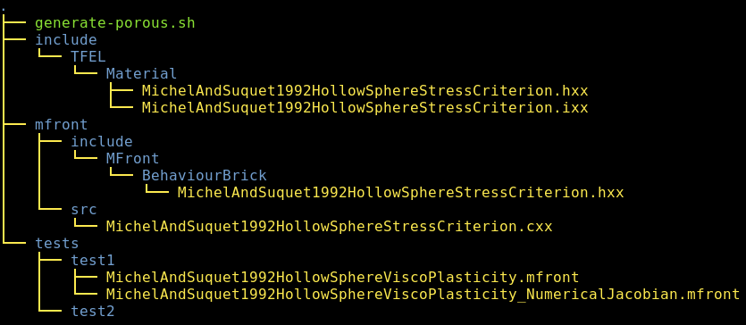
• PorousStressCriterionTemplate.hxx. Beware that this file is not the same as the one used in the first part of this document.
• PorousStressCriterionTemplate.cxx

The first file must be copied in a directory called mfront/include/MFront/BehaviourBrick and the second one in a directory called mfront/src subdirectory. Both must be renamed appropriately.

The working directory must now have the following structure:

As in the first part of this document, __Author__, __Date__, __StressCriterionName__ and __STRESS_CRITERION_NAME__ must be replaced by the appropriate values.

2.2 Adding the stress criterion options

In our case, the getOptions method must be implemented to declare the n material coefficient:

std::vector<OptionDescription> MichelAndSuquet1992HollowSphereTestStressCriterion::getOptions() const {
  auto opts = PorousStressCriterionBase::getOptions();
  opts.emplace_back("n", "Norton exponent of the matrix",
                    OptionDescription::MATERIALPROPERTY);
  return opts;
} // end of MichelAndSuquet1992HollowSphereTestStressCriterion::getOptions()

The getPorosityEffectOnEquivalentPlasticStrain method must be modified. But default, its returns the STANDARD_POROSITY_CORRECTION_ON_EQUIVALENT_PLASTIC_STRAIN value which would define define the increment of the viscoplastic strain as:

\[ \Delta\,\underline{\varepsilon}^{\mathrm{vp}}= {\left(1-f\right)}\,\Delta\,p\,\underline{n} \]

In the case of the stress criterion discussed in this tutorial, this \(1-f\) correction shall not be taken into account. Hence, the correct implementation for this method is:

StressCriterion::PorosityEffectOnFlowRule
MichelAndSuquet1992HollowSphereTestStressCriterion::getPorosityEffectOnEquivalentPlasticStrain() const {
  return StressCriterion::NO_POROSITY_EFFECT_ON_EQUIVALENT_PLASTIC_STRAIN;
}  // end of MichelAndSuquet1992HollowSphereTestStressCriterion::getPorosityEffectOnEquivalentPlasticStrain()

2.3 Compilation of the MFront plugin

Note

This paragraph assumes that you are working under a standard LiNuX environment. In particular, we assume that you use g++ as your C++ compiler. This can easily be changed to match your needs.

The MichelAndSuquet1992HollowSphereTestStressCriterion.cxx can now be compiled in a plugin as follows. Go in the mfront/src directory and type:

$ g++ -I ../include/ `tfel-config --includes `            \
      `tfel-config --oflags --cppflags --compiler-flags`  \
      -DMFRONT_ADITIONNAL_LIBRARY                         \
      `tfel-config --libs` -lTFELMFront                   \
      --shared -fPIC MichelAndSuquet1992HollowSphereTestStressCriterion.cxx         \
      -o libAdditionalStressCriteria.so

The calls to tfel-config allows retrieving the paths to the TFEL headers and libraries. The MFRONT_ADITIONNAL_LIBRARY flag activate a portion of the source file whose only purpose is to register the MichelAndSuquet1992HollowSphereTest stress criterion in an abstract factory.

2.4 Testing the plugin

To test the plugin, go in the tests/test2 directory.

Create a file MichelAndSuquet1992HollowSphereTestViscoPlasticity.mfront with the following content:

@DSL Implicit;

@Behaviour MichelAndSuquet1992HollowSphereTestViscoPlasticity;
@Author Thomas Helfer, Jérémy Hure, Mohamed Shokeir;
@Date 25 / 03 / 2020;
@Description {
}

@Algorithm NewtonRaphson;
@Epsilon 1.e-14;
@Theta 1;

@ModellingHypotheses{".+"};
@Brick StandardElastoViscoPlasticity{
  stress_potential : "Hooke" {
    young_modulus : 200e9,
    poisson_ratio : 0.3},
  inelastic_flow : "Norton" {
    criterion : "MichelAndSuquet1992HollowSphereTest" {
      n : 8},
    n: 8,
    K: 50e6,
    A: 1.e-4
  }
};

Note

Here, we see that the Norton exponent has to be repeated twice:

• one for the definition of the stress criterion.
• one for the definition of the Norton flow.

This is due to the structure, i.e. the abstractions, used by the brick which considers that the inelastic flow has now knowledge of the stress criterion.

This file can be compiled as follows:

$ MFRONT_ADDITIONAL_LIBRARIES=../../mfront/src/libAdditionalStressCriteria.so \
  mfront -I $(pwd)/../../include/ --obuild --interface=generic                \
  MichelAndSuquet1992HollowSphereTestViscoPlasticity.mfront

This implementation can be checked with the same MTest file than in the first part of this tutorial.

3 Applications to uranimum dioxyde viscoplastic behaviours

3.1 Implementation of Salvo’ viscoplastic behaviour

This behaviour has been described in [3].

@DSL Implicit;

@Behaviour Salvo2015ViscoplasticBehaviour;
@Material UO2;
@Author Thomas Helfer, Jérémy Hure, Mohamed Shokeir;
@Date 25 / 03 / 2020;
@Description {
  "Salvo, Maxime, Jérôme Sercombe, Thomas Helfer, Philippe Sornay, and Thierry Désoyer. "
  "Experimental Characterization and Modeling of UO2 Grain Boundary Cracking at High "
  "Temperatures and High Strain Rates."
  "Journal of Nuclear Materials 460 (May 2015): 184–99."
  "https://doi.org/10.1016/j.jnucmat.2015.02.018."
}

@StrainMeasure Hencky;

@Algorithm NewtonRaphson;
@Epsilon 1.e-14;
@Theta 1;

//! Reference stress
@Parameter stress s0 = 5e6;
//! Activation temperature
// This temperature is equal to the activation energy (482 kJ/mol/K)
// divided by the ideal gas constant.
@Parameter temperature Ta = 57971.27513059395;
//! Reference strain rate
@Parameter strainrate de0 = 29.130;

@ModellingHypotheses{".+"};
@Brick StandardElastoViscoPlasticity{
  stress_potential : "Hooke" {
    young_modulus : "UO2_YoungModulus.mfront",
    poisson_ratio : "UO2_PoissonRatio.mfront"},
  inelastic_flow : "HyperbolicSine" {
    criterion : "MichelAndSuquet1992HollowSphereTest" {
      n : 6},
    K: "s0",
    A: "de0 * exp(-Ta/T)"
  }
};

Note

This implementation has been proposed as an example of how the brick can be used in practice. This implementation barely compiles at this stage and shall be carefully verified before any usage in a fuel performance code.

3.2 Coupling of the Salvo’ viscoplastic behaviour with the DDIF2 damage law

The DDIF2 damage law is currently the standard damage law used in CEA’ fuel performance codes (see [4–6] for a complete description). Coupling of the Salvo’ viscoplastic behaviour with the DDIF2 damage law boils downs to replacing the Hooke stress potential with the DDIF2 stress potential, as follows:

@DSL Implicit;

@Behaviour DDIF2Salvo2015ViscoplasticBehaviour;
@Material UO2;
@Author Thomas Helfer, Jérémy Hure, Mohamed Shokeir;
@Date 25 / 03 / 2020;
@Description {
  "Salvo, Maxime, Jérôme Sercombe, Thomas Helfer, Philippe Sornay, and Thierry Désoyer. "
  "Experimental Characterization and Modeling of UO2 Grain Boundary Cracking at High "
  "Temperatures and High Strain Rates."
  "Journal of Nuclear Materials 460 (May 2015): 184–99."
  "https://doi.org/10.1016/j.jnucmat.2015.02.018."
}

@StrainMeasure Hencky;

@Algorithm NewtonRaphson;
@Epsilon 1.e-14;
@Theta 1;

//! Reference stress
@Parameter stress s0 = 5e6;
//! Activation temperature
// This temperature is equal to the activation energy (482 kJ/mol/K)
// divided by the ideal gas constant.
@Parameter temperature Ta = 57971.27513059395;
//! Reference strain rate
@Parameter strainrate de0 = 29.130;

@ModellingHypotheses{".+"};
@Brick StandardElastoViscoPlasticity{
  stress_potential : "DDIF2" {
    young_modulus : "UO2_YoungModulus.mfront",
    poisson_ratio : "UO2_PoissonRatio.mfront",
    fracture_stress : "UO2_ElasticLimit.mfront",
    fracture_energy : "UO2_FractureEnergy.mfront"
  },
  inelastic_flow : "HyperbolicSine" {
    criterion : "MichelAndSuquet1992HollowSphereTest" {
      n : 6},
    K: "s0",
    A: "de0 * exp(-Ta/T)"
  }
};

References