Burger_EDF_CIWAP_2021 constitutive
law for concrete creep and shrinkageThis document introduces the Burger_EDF_CIWAP_2021 which
aims at modelling the following phenomena in concrete:
It is an isotropic constitutive law for all phenomena.
Two variants, described in this document, of the implementation of
this behaviour are available in the MFrontGallery
project:
The ACES project and the VERCORS benchmark
The
Burger_EDF_CIWAP_2021is shared on the MFront gallery in the framework of the European project ACES [1, 2], in order to give acces to the VERCORS benchmark 3rd participants [3].
The Burger mechanical model was originally developed for
EDF R&D by [4–6]. It was
then modified in order to better represent long term basic creep
according to [7], and implemented as a
code_aster law and then in MFront.
The version of the law described in the present document and named
Burger_EDF_CIWAP_2021 is different from the one implemented
in code_aster, which is described in [6], on two points:
The total strain is the sum of 4 components:
\[ \underline{\varepsilon}^{\mathrm{to}}= \underline{\varepsilon}^{\mathrm{el}}+ \underline{\varepsilon}^{\text{shr}} + \underline{\varepsilon}^{\text{bc}} + \underline{\varepsilon}^{\text{dc}} \qquad{(1)}\]
where:
The variation of drying shrinkage \({\dot{\underline{\varepsilon}}}^{\text{shr}}\) is considered proportional to the variation of relative humidity \(\dot{h}\):
\[ \dot{\underline{\varepsilon}}^{\text{shr}} = \dot{\underline{\varepsilon}}^{\text{shr}}\,\underline{I} = k^{\text{shr}}\dot{h}\,\underline{I} \qquad{(2)}\]
The combination of elastic and basic creep strains is known as a Burger rheological model. Elasticity and basic creep are isotropic and hence, the Burger model is duplicated in deviatoric and spherical chains (“d” relates to deviatoric while “s” relates to spherical).
For each chain the strain is composed of elastic strain (\(\varepsilon_{s}^{\text{el}}\) and \(\underline{\varepsilon}_{d}^{\text{el}}\)), reversible basic creep modeled by the Kelvin-Voigt element (\(\varepsilon_{s}^{\text{rbc}}\) and \(\underline{\varepsilon}_{d}^{\text{rbc}}\)) and irreversible basic creep modeled by the Maxwell element by using a viscosity which is not constant in time and dependent on the current state of strain (\(\varepsilon_{s}^{\text{ibc}}\) and \(\underline{\varepsilon}_{d}^{\text{ibc}}\)):
\[ \underline{\varepsilon}^{\text{bc}}=\underline{\varepsilon}^{\text{rbc}}+\underline{\varepsilon}^{\text{ibc}}= \varepsilon_{s}^{\text{rbc}}\,\underline{I}+\underline{\varepsilon}_{d}^{\text{rbc}}+ \varepsilon_{s}^{\text{ibc}}\,\underline{I}+\underline{\varepsilon}_{d}^{\text{ibc}} \]
The equations related to this Burger model are now recalled for the spherical chain (the deviatoric can be obtained by replacing “s” by “d” and using tensors instead of scalars).
The elastic strain is simply proportional to the stress (here written using the elastic bulk modulus \(k^{\text{el}}\) and shear coefficient \(\mu^{\text{el}}\) :
\[ \left\{ \begin{aligned} \varepsilon_{s}^{\text{el}} &= \frac{1}{3\,k^{\text{el}}}\,p\\ \underline{\varepsilon}_{d}^{\text{el}} &= \frac{1}{2\,\mu^{\text{el}}}\,\underline{\sigma}_{d} \end{aligned} \right. \qquad{(3)}\]
The basic creep strains are assumed proportional to the relative humidity. The reversible basic creep is governed by the equation:
\[ h\,p = k^{\text{rs}}\,\varepsilon_{s}^{\text{rbc}} + \eta^{\text{rs}}\,{\dot{\varepsilon}}_{s}^{\text{rbc}} \qquad{(4)}\]
while the irreversible basic creep follows the equation:
\[ h\,p = \eta^{\text{is}}{\dot{\varepsilon}}_{s}^{\text{ibc}} \qquad{(5)}\]
The viscosity of the irreversible contribution is assumed to be dependent on the current state of irreversible strains following the equation:
\[\eta^{\text{is}} = \eta_{0}^{\text{is}}\exp{\left( \frac{\left\|\underline{\varepsilon}_{m}^{\text{ibc}}\right\|}{\kappa} \right)}\]
where \(\left\|\underline{\varepsilon}_{m}^{\text{ibc}}\right\|= \max_{\tau\in[0,t]}\sqrt{\underline{\varepsilon}^{\text{ibc}}{\left(\tau\right)}\,\colon\,\underline{\varepsilon}^{\text{ibc}}{\left(\tau\right)}}\).
This feature induces non-linearity in the creep model. The treatment of this non-linearity is one of the most involved aspect of the proposed implementation and will be detailed in Section 2.3.
The model is also thermo-activated by adding a temperature dependence to the parameters of the previous equations. Parameters \(k^{\text{rs}}\), \(k^{\text{rd}}\), \(\eta^{\text{rs}}\), \(\eta^{\text{rd}}\), \(\eta^{\text{is}}\) and \(\eta^{\text{id}}\) have the following temperature dependence exemplified on \(k^{\text{rs}}\):
\[ k^{\text{rs}}{\left( T \right)} = k_{0}^{\text{rs}}\exp{\left( \frac{Q}{R}{\left( \frac{1}{T} - \frac{1}{T_{0}} \right)} \right)} \qquad{(6)}\]
Also,
\[ \kappa = {{\displaystyle \frac{\displaystyle \kappa_{0}}{\displaystyle \exp{\left( \frac{Q}{R}{\left( \frac{1}{T} - \frac{1}{T_{0}} \right)} \right)}}}} \qquad{(7)}\]
where \(Q\) is the activation energy for creep.
Finally, the desiccation creep is computed according to a modified version of a law called Bažant’s law, relating the excess of strain rate during drying to the rate of change of the water concentration [9]. It is supposed in this version of the model that desiccation creep occurs with a zero Poisson’s ratio and that its rate is proportional to the absolute value of the relative humidity rate. Also, following a proposition by Boucher [8, 10] taking inspiration in Benboudjema [4] who noted that the behavior is not symmetric between drying and imbibition. Here the imbibition desiccation strain is considered negligible. Also, the desiccation creep occurs only during first drying down to a given relative humidity.
\[ \dot{\underline{\varepsilon}}^{\text{dc}} = \frac{1}{\eta_{\text{fd}}}\underline{\sigma}\left\langle \dot{h} \right\rangle \qquad{(8)}\]
where:
\[ \langle\dot{h}\rangle = \left\{ \begin{aligned} \dot{h} &\quad\text{if}\quad \dot{h} < 0 \quad\text{and}\quad h{\left(t\right)} < \min_{\tau\in [0,t]} h{\left(\tau\right)}\\ 0 &\quad\text{otherwise} \end{aligned} \right. \]
To integrate this behaviour, we use an implicit scheme described in this page [11]. This scheme turns the constitutive equations, which forms a system of ordinary differential equations, into a system of non linear equations.
Such scheme is usually more efficient than explicit integration schemes based on (explicit) Runge-Kutta methods and allows deriving the consistent tangent operator which can lead to a quadratic convergence of the equilibrium at the global scale.
A standard Newton-Raphson algorithm will be used to find the solution of the implici system, which requires to compute the jacobian of the implicit system.
The role of the implicit scheme is to determine the following increments:
\[ \Delta\,\underline{\varepsilon}^{\mathrm{el}},\,\Delta\,\underline{\varepsilon}^{\text{shr}},\, \Delta\,\underline{\varepsilon}^{\text{bc}},\,\Delta\,\underline{\varepsilon}^{\text{dc}},\,\Delta\,\left\|\underline{\varepsilon}_{m}^{\text{ibc}}\right\| \]
For convenience, the basic creep contribution \(\underline{\varepsilon}^{\text{bc}}\) is explicitly slitted into its reverible \(\underline{\varepsilon}^{\text{rbc}}\) and irreversible part \(\underline{\varepsilon}^{\text{ibc}}\). The set of increments to be determined is then:
\[ \Delta\,\underline{\varepsilon}^{\mathrm{el}},\,\Delta\,\underline{\varepsilon}^{\text{shr}}, \,\Delta\,\underline{\varepsilon}^{\text{rbc}}, \,\Delta\,\underline{\varepsilon}^{\text{ibc}},\,\Delta\,\underline{\varepsilon}^{\text{dc}},\,\Delta\,\left\|\underline{\varepsilon}_{m}^{\text{ibc}}\right\| \]
For one of those increments, one can either, as shown below:
MFront does not automatically defines the increment
associated with an auxiliary state variable.From an numerical point of view, using an auxiliary state variable rather than a state variable is interesting as it reduces the size of the implicit system to be solved. However, it generally leads to more complex implementations.
For reasons that will become clearer later when we will examine each contributions, we choose the following set of state variables:
\[ \underline{\varepsilon}^{\mathrm{el}}, \underline{\varepsilon}^{\text{ibc}}, \left\|\underline{\varepsilon}_{m}^{\text{ibc}}\right\| \]
and the following set of auxiliary state variables:
\[ \underline{\varepsilon}^{\text{shr}}, \underline{\varepsilon}^{\text{rbc}}, \underline{\varepsilon}^{\text{dc}} \]
In the proposed implementation, each inelastic strain will be split into its spherical and deviatoric part for the sake of clarity. With this choice, the final set of state variables is:
\[ \underline{\varepsilon}^{\mathrm{el}}, \varepsilon_{s}^{\text{ibc}}, \underline{\varepsilon}_{d}^{\text{ibc}}, \left\|\underline{\varepsilon}_{m}^{\text{ibc}}\right\| \]
and the following set of auxiliary state variables:
\[ \underline{\varepsilon}^{\text{shr}}, \varepsilon_{s}^{\text{rbc}}, \underline{\varepsilon}_{d}^{\text{rbc}}, \underline{\varepsilon}^{\text{dc}} \]
Drawbacks of this choice are an increase the size of the implicit system and a higher memory consumption (i.e. the number of values saved from one time step to the other).
This choice can easily be reverted, leading to a more compact and efficient implementation, while a bit less readable.
State variables are automatically updated when the solutions (the
increment of the state variables) of the implicit equations are found.
Auxiliary state variables are generally updated in a dedicated code
block called @UpdateAuxiliaryStateVariables.
For this behaviour, declaring the auxiliary state variables is
convenient for post-processing, i.e. the behaviour integration only
requires to determine their increments during the time step and does not
require to know their values at the beginning of the time step. If such
post-processing does not matter, a significant amount of memory can be
saved by removing their declaration as auxiliary state variables and
their update in the @UpdateAuxiliaryStateVariable code
block.
The stress tensor is a function of the increment of the elastic strain \(\underline{\varepsilon}^{\mathrm{el}}\). Its value at the middle of the time step (at \(t+\theta\,\Delta\,t\)) is given by:
\[ \left\{ \begin{aligned} {\left.p\right|_{t+\theta\,\Delta\,t}} &= {\left(3\,{\left.\lambda^{\text{el}}\right|_{t+\theta\,\Delta\,t}}+2\,{\left.\mu^{\text{el}}\right|_{t+\theta\,\Delta\,t}}\right)}\,{\left.\varepsilon^{\text{el}}_{s}\right|_{t+\theta\,\Delta\,t}} &= 3\,{\left.k^{\text{el}}\right|_{t+\theta\,\Delta\,t}}\,{\left.\varepsilon^{\text{el}}_{s}\right|_{t+\theta\,\Delta\,t}} \\ {\left.\underline{\sigma}_d\right|_{t+\theta\,\Delta\,t}} &= 2\,{\left.\mu^{\text{el}}\right|_{t+\theta\,\Delta\,t}}\,{\left.\underline{\varepsilon}^{\mathrm{el}}_{d}\right|_{t+\theta\,\Delta\,t}} \end{aligned} \right. \qquad{(9)}\]
The derivatives of the pressure and the deviatoric stress with regard to the elastic strain increment are thus:
\[ {\displaystyle \frac{\displaystyle \partial {\left.p\right|_{t+\theta\,\Delta\,t}}}{\displaystyle \partial \Delta\,\underline{\varepsilon}^{\mathrm{el}}}} = 3\,\theta\,{\left.k^{\text{el}}\right|_{t+\theta\,\Delta\,t}}\,\underline{I} \quad\text{and}\quad {\displaystyle \frac{\displaystyle \partial {\left.\underline{\sigma}_d\right|_{t+\theta\,\Delta\,t}}}{\displaystyle \partial \Delta\,\underline{\varepsilon}^{\mathrm{el}}}} = 2\,\theta\,{\left.\mu^{\text{el}}\right|_{t+\theta\,\Delta\,t}}\,\underline{\underline{\mathbf{K}}} \qquad{(10)}\]
Equation (4) can be discretized as follows:
\[ \begin{aligned} &&k^{\text{rs}}\,{\left.\varepsilon_{s}^{\text{rbc}}\right|_{t+\theta\,\Delta\,t}} + \eta^{\text{rs}}\,{{\displaystyle \frac{\displaystyle \Delta\,\varepsilon_{s}^{\text{rbc}}}{\displaystyle \Delta\,t}}}&={\left.h\right|_{t+\theta\,\Delta\,t}}\,{\left.p\right|_{t+\theta\,\Delta\,t}}\\ &\Rightarrow&{\left(\eta^{\text{rs}}+\theta\,\Delta\,t\,k^{\text{rs}}\right)}\,\Delta\,\varepsilon_{s}^{\text{rbc}}&=\Delta\,t\,{\left.h\right|_{t+\theta\,\Delta\,t}}\,{\left.p\right|_{t+\theta\,\Delta\,t}}-\Delta\,t\,k^{\text{rs}}\,{\left.\varepsilon_{s}^{\text{rbc}}\right|_{t}} \end{aligned} \]
Finally, the expression of the increment of the reversible part of the basic creep is:
\[ \Delta\,\varepsilon_{s}^{\text{rbc}} = \Delta\,t\,{{\displaystyle \frac{\displaystyle {\left.h\right|_{t+\theta\,\Delta\,t}}}{\displaystyle \eta^{\text{rs}}+\theta\,\Delta\,t\,k^{\text{rs}}}}}\,{\left.p\right|_{t+\theta\,\Delta\,t}}- \Delta\,t\,{{\displaystyle \frac{\displaystyle k^{\text{rs}}}{\displaystyle \eta^{\text{rs}}+\theta\,\Delta\,t\,k^{\text{rs}}}}}\,{\left.\varepsilon_{s}^{\text{rbc}}\right|_{t}} \qquad{(11)}\]
This equation shows that \(\Delta\,\varepsilon_{s}^{\text{rbc}}\) is a simple linear function of the pressure, i.e. a simple function of the elastic strain increment.
The derivative of \(\Delta\,\varepsilon_{s}^{\text{rbc}}\) with respect to the elastic strain increment is simply:
\[ {\displaystyle \frac{\displaystyle \partial \Delta\,\varepsilon_{s}^{\text{rbc}}}{\displaystyle \partial \Delta\,\underline{\varepsilon}^{\mathrm{el}}}}= \Delta\,t\,{{\displaystyle \frac{\displaystyle {\left.h\right|_{t+\theta\,\Delta\,t}}}{\displaystyle \eta^{\text{rs}}+\theta\,\Delta\,t\,k^{\text{rs}}}}}\,{\displaystyle \frac{\displaystyle \partial {\left.p\right|_{t+\theta\,\Delta\,t}}}{\displaystyle \partial \Delta\,\underline{\varepsilon}^{\mathrm{el}}}} \]
where the derivative \({\displaystyle \frac{\displaystyle \partial {\left.p\right|_{t+\theta\,\Delta\,t}}}{\displaystyle \partial \Delta\,\underline{\varepsilon}^{\mathrm{el}}}}\) is given by Equation (10).
Equation (5) can be discretized as follows:
\[ \Delta\,\varepsilon_{s}^{\text{ibc}} = \Delta\,t\,{{\displaystyle \frac{\displaystyle {\left.h\right|_{t+\theta\,\Delta\,t}}}{\displaystyle \eta^{\text{is}}{\left({\left.\left\|\underline{\varepsilon}_{m}^{\text{ibc}}\right\|\right|_{t+\theta\,\Delta\,t}}\right)}}}}\,{\left.p\right|_{t+\theta\,\Delta\,t}} \]
The implicit equation \(f_{\Delta\,\varepsilon_{s}^{\text{ibc}}}\) associated with \(\Delta\,\varepsilon_{s}^{\text{ibc}}\) is thus:
\[ f_{\Delta\,\varepsilon_{s}^{\text{ibc}}} = \Delta\,\varepsilon_{s}^{\text{ibc}}- \Delta\,t\,{{\displaystyle \frac{\displaystyle {\left.h\right|_{t+\theta\,\Delta\,t}}}{\displaystyle \eta^{\text{is}}{\left({\left.\left\|\underline{\varepsilon}_{m}^{\text{ibc}}\right\|\right|_{t+\theta\,\Delta\,t}}\right)}}}}\,{\left.p\right|_{t+\theta\,\Delta\,t}} \]
The following derivatives will be useful:
\[ \left\{ \begin{aligned} {\displaystyle \frac{\displaystyle \partial f_{\Delta\,\varepsilon_{s}^{\text{ibc}}}}{\displaystyle \partial \Delta\,\varepsilon_{s}^{\text{ibc}}}} &= 1 \\ {\displaystyle \frac{\displaystyle \partial f_{\Delta\,\varepsilon_{s}^{\text{ibc}}}}{\displaystyle \partial \Delta\,\underline{\varepsilon}^{\mathrm{el}}}} &= - \Delta\,t\,{{\displaystyle \frac{\displaystyle {\left.h\right|_{t+\theta\,\Delta\,t}}}{\displaystyle \eta^{\text{is}}{\left({\left.\left\|\underline{\varepsilon}_{m}^{\text{ibc}}\right\|\right|_{t+\theta\,\Delta\,t}}\right)}}}}\,{\displaystyle \frac{\displaystyle \partial {\left.p\right|_{t+\theta\,\Delta\,t}}}{\displaystyle \partial \underline{\varepsilon}^{\mathrm{el}}}} \\ {\displaystyle \frac{\displaystyle \partial f_{\Delta\,\varepsilon_{s}^{\text{ibc}}}}{\displaystyle \partial \Delta\,{\left.\left\|\underline{\varepsilon}_{m}^{\text{ibc}}\right\|\right|_{t+\theta\,\Delta\,t}}}} &= \Delta\,t\,{{\displaystyle \frac{\displaystyle {\left.h\right|_{t+\theta\,\Delta\,t}}}{\displaystyle {\left(\eta^{\text{is}}{\left({\left.\left\|\underline{\varepsilon}_{m}^{\text{ibc}}\right\|\right|_{t+\theta\,\Delta\,t}}\right)}\right)}^{2}}}}\,{\left.p\right|_{t+\theta\,\Delta\,t}}\, {\displaystyle \frac{\displaystyle \partial \eta^{\text{is}}}{\displaystyle \partial \Delta\,\left\|\underline{\varepsilon}_{m}^{\text{ibc}}\right\|}} \\ \end{aligned} \right. \]
In this document, we choose the following implicit equation to determine \(\Delta\,\left\|\underline{\varepsilon}_{m}^{\text{ibc}}\right\|\):
\[ f_{\left\|\underline{\varepsilon}_{m}^{\text{ibc}}\right\|}= \left\{ \begin{aligned} {\left.\left\|\underline{\varepsilon}_{m}^{\text{ibc}}\right\|\right|_{t}}+\Delta\,\left\|\underline{\varepsilon}_{m}^{\text{ibc}}\right\|- \sqrt{{\left.\underline{\varepsilon}^{\text{ibc}}\right|_{t+\Delta\,t}}\,\colon\,{\left.\underline{\varepsilon}^{\text{ibc}}\right|_{t+\Delta\,t}}} &\quad\text{if}\quad \sqrt{{\left.\underline{\varepsilon}^{\text{ibc}}\right|_{t+\Delta\,t}}\,\colon\,{\left.\underline{\varepsilon}^{\text{ibc}}\right|_{t+\Delta\,t}}}>{\left.\left\|\underline{\varepsilon}_{m}^{\text{ibc}}\right\|\right|_{t}}&\\ \Delta\,\left\|\underline{\varepsilon}_{m}^{\text{ibc}}\right\|&\quad\text{otherwise}& \end{aligned} \right. \qquad{(12)}\]
The derivatives of this equation are:
\[ \left\{ \begin{aligned} {\displaystyle \frac{\displaystyle \partial f_{\left\|\underline{\varepsilon}_{m}^{\text{ibc}}\right\|}}{\displaystyle \partial \Delta\,\left\|\underline{\varepsilon}_{m}^{\text{ibc}}\right\|}} &= 1\\ {\displaystyle \frac{\displaystyle \partial f_{\left\|\underline{\varepsilon}_{m}^{\text{ibc}}\right\|}}{\displaystyle \partial \Delta\,\underline{\varepsilon}^{\text{ibc}}}} &= -{{\displaystyle \frac{\displaystyle \Delta\,\underline{\varepsilon}^{\text{ibc}}}{\displaystyle \sqrt{{\left.\underline{\varepsilon}^{\text{ibc}}\right|_{t+\Delta\,t}}\,\colon\,{\left.\underline{\varepsilon}^{\text{ibc}}\right|_{t+\Delta\,t}}}}}}\quad\text{if}\quad \sqrt{{\left.\underline{\varepsilon}^{\text{ibc}}\right|_{t+\Delta\,t}}\,\colon\,{\left.\underline{\varepsilon}^{\text{ibc}}\right|_{t+\Delta\,t}}}>{\left.\left\|\underline{\varepsilon}_{m}^{\text{ibc}}\right\|\right|_{t}}\\ \end{aligned} \right. \]
Using Implicit Equation (12) may lead to spurious oscillations of the Newton algorithm, although this is not observered in the test cases below.
This is due to the fact that the derivatives of this equation are not continuous.
A standard way to overcome this issue is to use a status method which
can be implemented in MFront [12].
In this paragraph, we introduce an alternative treatment of this equation based on the regularised Fisher-Burmeister complementary function \(\Phi_{\varepsilon_{\text{FB}}}\), introduced in [13] and whose application to plasticity is described on a dedicated web page [14]:
\[ \Phi_{\varepsilon}{\left(x,y\right)}=x+y-\sqrt{x^{2}+y^{2}+\varepsilon_{\text{FB}}^{2}} \]
where \(\varepsilon_{\text{FB}}\) denotes a small numerical parameter.
\(\Phi_{\varepsilon}{\left(x,y\right)}\) has the following property:
\[ \Phi_{\varepsilon}{\left(x,y\right)}=0 \quad\Leftrightarrow\quad \left\{ \begin{aligned} x&\geq 0\\ y&\geq 0\\ 2\,x\,y&=\varepsilon^{2} \end{aligned} \right. \qquad{(13)}\]
Based on Property (13), the Implicit Equation (12) can be replaced by the following equation:
\[ f_{\left\|\underline{\varepsilon}_{m}^{\text{ibc}}\right\|}=\Phi_{\varepsilon_{\text{FB}}}{\left(\Delta\,\left\|\underline{\varepsilon}_{m}^{\text{ibc}}\right\|, {\left.\left\|\underline{\varepsilon}_{m}^{\text{ibc}}\right\|\right|_{t}}+\Delta\,\left\|\underline{\varepsilon}_{m}^{\text{ibc}}\right\|- \sqrt{{\left.\underline{\varepsilon}^{\text{ibc}}\right|_{t+\Delta\,t}}\,\colon\,{\left.\underline{\varepsilon}^{\text{ibc}}\right|_{t+\Delta\,t}}}\right)} \qquad{(14)}\]
Implicit Equation (14) has continuous derivatives.
\(\Phi_{\varepsilon}\) and its
derivatives are implemented in the TFEL/Math library in Version 3.2 but their usage requires to include the TFEL/Math/FischerBurmeister.hxx
header:
regularisedFischerBurmeisterFunction function
implements the computation of \(\Phi_{\varepsilon}\).regularisedFischerBurmeisterFunctionFirstDerivatives
function implements the computation of the derivatives of \({\displaystyle \frac{\displaystyle \partial
\Phi_{\varepsilon}}{\displaystyle \partial x}}\) and \({\displaystyle \frac{\displaystyle \partial
\Phi_{\varepsilon}}{\displaystyle \partial y}}\).Equation (8) can be discretized as follows:
\[ \Delta\,\underline{\varepsilon}^{\text{dc}} = \frac{\Delta\,t}{\eta_{\text{fd}}}\left\langle \dot{h} \right\rangle\,{\left.\underline{\sigma}\right|_{t+\theta\,\Delta\,t}} \]
\(\Delta\,\underline{\varepsilon}^{\text{dc}}\) is thus a simple function of the elastic strain increment \(\Delta\,\underline{\varepsilon}^{\mathrm{el}}\).
Its derivative with respect to the elastic strain increment is:
\[ {\displaystyle \frac{\displaystyle \partial \Delta\,\underline{\varepsilon}^{\text{dc}}}{\displaystyle \partial \Delta\,\underline{\varepsilon}^{\mathrm{el}}}} =\frac{\Delta\,t}{\eta_{\text{fd}}}\left\langle \dot{h} \right\rangle\,{\displaystyle \frac{\displaystyle \partial {\left.\underline{\sigma}\right|_{t+\theta\,\Delta\,t}}}{\displaystyle \partial \Delta\,\underline{\varepsilon}^{\mathrm{el}}}} =\frac{\Delta\,t}{\eta_{\text{fd}}}\left\langle \dot{h} \right\rangle\, {\left(\underline{I}\,\otimes\,{\displaystyle \frac{\displaystyle \partial {\left.p\right|_{t+\theta\,\Delta\,t}}}{\displaystyle \partial \Delta\,\underline{\varepsilon}^{\mathrm{el}}}}+ {\displaystyle \frac{\displaystyle \partial {\left.\underline{\sigma}_{d}\right|_{t+\theta\,\Delta\,t}}}{\displaystyle \partial \Delta\,\underline{\varepsilon}^{\mathrm{el}}}}\right)} \]
The implicit equation \(f_{\underline{\varepsilon}^{\mathrm{el}}}\) associated with the elastic strain increment is given by the split of the strain (1) written in incremental form:
\[ f_{\underline{\varepsilon}^{\mathrm{el}}}=\Delta\,\underline{\varepsilon}^{\mathrm{el}}-\Delta\,\underline{\varepsilon}^{\mathrm{to}} +\Delta\,\underline{\varepsilon}^{\text{shr}} +\Delta\,\underline{\varepsilon}^{\text{bc}} +\Delta\,\underline{\varepsilon}^{\text{dc}} \qquad{(15)}\]
MFront implementationsStandardElasticity
brickThe domain specific language (DSL) suitable for implementing an
implicit scheme based on standard strain-based beahviour is called Implicit [11].
The @DSL keyword allows specifying the domain specific
language to be used:
@DSL Implicit;The standard elasticity brick [15] is appropriate for this behaviour which provides additional functionnalities such as:
The usage of the StandardElasticity is introduced as
follows:
@Brick StandardElasticity;Automic declaration of the elastic strain
The
ImplicitDSL automatically defines the elastic strain as the first state variable.
The main steps of the behaviour integration used by the
Implicit DSL are reported on Figure 1:
@InitLocalVariables code block is called once
before the beginning of the Newton-Raphson algorithm.@ComputeStress which is meant to update the estimate of
the stress at the middle of the time step \({\left.\underline{\sigma}\right|_{t+\theta\,\Delta\,t}}\).
This code block is automatically added by the
StandardElasticity brick.@Integrator is meant to built the implicit equations
and its derivatives.@AdditionalConvergenceChecks is meant to add additional
convergence checks. This code block is not considered in this
document.ComputeFinalStress which computes the stress at the end
of the time step. This code block is automatically added by the
StandardElasticity brick.@UpdateAuxiliaryStateVariables which is meant to update
the auxiliary state variables.@TangentOperator which is meant to compute the tangent
operators. This code block is automatically added by the
StandardElasticity brick.The @Behaviour keyword is required to name the
behaviour, as follows:
@Behaviour Burger_EDF_CIWAP_2021;The @Material keyword allows to associate the behaviour
to material:
@Material Concrete;The @Author keyword gives the name of the person who
implemented the behaviour:
@Author François Hamon (EDF R&D ERMES - T65),
        Jean - Luc Adia (EDF R&D MMC - T25),
        Thomas Helfer (CEA IRESNE/DES/DEC/SESC);
The @Description keyword allows to introduce a small
description of the implementation:
@Description {
`Burger_EDF_CIWAP_2021` model for concrete creep;
Compater to `code_aster`' `BETON_BURGER` constitutive equations, this behaviour
takes into account two points:
-adding of shrinkage depending to relative humidity;
-drying creep depending to the positive part of derivative of relative humidity;
}For this implementation, we will use the standard Newton-Raphson:
@Algorithm NewtonRaphson;The @Epsilon keyword allows to specify the default value
of the stopping criteria:
@Epsilon 1e-14;This default value can be changed at runtime using the
epsilon parameter.
The @Theta keyword allows the specify the default value
of the \(\theta\) parameter of the
implicit scheme:
@Theta 1;This default value can be changed at runtime using the
theta parameter.
If we want to use the alternative implicit equation for \(\Delta\,\left\|\underline{\varepsilon}_{m}^{\text{ibc}}\right\|\),
discussed in Section 2.3.4, we need to include the following header file
using the @Includes keyword:
@Includes{
#include "TFEL/Math/FischerBurmeister.hxx"
}Material properties are a classical way to create behaviours that can be used to describe a wide range of materials. Material properties are provided by the calling solver and are generally read in the input file.
MFront variable |
Description |
|---|---|
young |
Young modulus \(E^{\text{el}}\) |
nu |
Poisson ratio \(\nu^{\text{el}}\) |
K_SH |
Shrinkage coefficient \(k^{\text{shr}}\) |
K_RS |
Spherical reversible basic creep stiffness \(k_{0}^{\text{rs}}\) |
ETA_RS |
Spherical reversible basic creep viscosity \(\eta_{0}^{\text{rs}}\) |
KAPPA |
Reference strain for evolution of irreversible creep viscosity \(\kappa_{0}\) |
ETA_IS |
Spherical irreversible creep viscosity \(\eta_{0}^{\text{is}}\) |
K_RD |
Deviatoric reversible basic creep stiffness \(k_{0}^{\text{rd}}\) |
ETA_RD |
Deviatoric reversible basic creep viscosity \(\eta_{0}^{\text{rd}}\) |
ETA_ID |
Deviatoric irreversible creep viscosity \(\eta_{0}^{\text{id}}\) |
QSR_K |
Activation energy \(\frac{Q}{R}\) |
TEMP_0_C |
Reference temperature \(T_{0}\) |
ETA_FD |
Drying creep coefficient \(\eta_{\text{fd}}\) |
The material properties required by the
Burger_EDF_CIWAP_2021 behaviour are listed in Table 1.
Material properties are declared using the
@MaterialProperty keyword, as follows:
//! Elastic Young Modulus
@MaterialProperty stress young;
young.setGlossaryName("YoungModulus");
//! Elastic Poisson Ratio
@MaterialProperty real nu;
nu.setGlossaryName("PoissonRatio");
//! Shrinkage coefficient
@MaterialProperty real K_SH;
K_SH.setEntryName("ShrinkageFactor");
//! Spherical reversible basic creep stiffness
@MaterialProperty real K_RS;
K_RS.setEntryName("SphericReversibleStiffness");
//! Spherical reversible basic creep viscosity
@MaterialProperty real ETA_RS;
ETA_RS.setEntryName("SphericReversibleViscosity");
//! Reference strain for evolution of irreversible creep viscosity
@MaterialProperty real KAPPA;
KAPPA.setEntryName("IrreversibleCreepViscosityReferenceStrain");
//! Spherical irreversible creep viscosity
@MaterialProperty real ETA_IS;
ETA_IS.setEntryName("SphericIrreversibleCreepViscosity");
//! Deviatoric reversible basic creep stiffness
@MaterialProperty real K_RD;
K_RD.setEntryName("DeviatoricReversibleStiffness");
//! Deviatoric reversible basic creep viscosity
@MaterialProperty real ETA_RD;
ETA_RD.setEntryName("DeviatoricReversibleViscosity");
//! Deviatoric irreversible creep viscosity
@MaterialProperty real ETA_ID;
ETA_ID.setEntryName("DeviatoricIrreversibleViscosity");
//! Activation energy of basic creep parameter
@MaterialProperty real QSR_K;
QSR_K.setEntryName("ActivationEnergy");
//! Reference temperature for temperature activation of basic creep
@MaterialProperty real TEMP_0_C;
TEMP_0_C.setEntryName("ReferenceTemperature");
//! Drying creep viscosity
@MaterialProperty real ETA_FD;
ETA_FD.setEntryName("DryingCreepVicosity");
Note that we associated to each material property an external name
(either a glossary name or a so-called entry name) using the
setGlossaryName or setEntryName methods. The
external name is the name of this variable as seen by the calling solver
and its user when this solver supports deep integration of
MFront behaviours.
Glossary names are a restricted list of names described on a dedicated page [16]. The setGlossaryName
fails if the given name is not in this list, avoiding typing errors.
Material properties vs parameters
In most MFront tutorials, we usually prefer to use parameters, which are declared using the
@Parameterkeyword.Contrary to material properties, parameters have default values. Parameters are thus useful to build behaviours specific to one particular material. Such behaviours are self-contained, which considerably eases building a strict material knowledge management policy.
Parameters are also stored in a global structure. This means that parameters are uniform. In some codes, material properties may be defined on a per integration point basis.
MFront variable |
Description |
|---|---|
ELIM |
Limit strain for the irreversible creep model |
ESPHI |
Spherical irreversible basic reep strain \(\varepsilon_{s}^{\text{ibc}}\) |
EDEVI |
Deviatoric irreversible basic creep strain \(\varepsilon_{d}^{\text{ibc}}\) |
Following Section 2.1, the state variables required by the
Burger_EDF_CIWAP_2021 behaviour are listed in Table 2.
The state variables are introduced by the @StateVariable
as follows:
@StateVariable strain ELIM;
ELIM.setEntryName("MaximumValueOfTheIrreversibleStrain");
//! Spherical irreversible basic creep strain
@StateVariable strain ESPHI;
ESPHI.setEntryName("SphericIrreversibleStrain");
//! Deviatoric irreversible basic creep strain
@StateVariable StrainStensor EDEVI;
EDEVI.setEntryName("DeviatoricIrreversibleStrain");MFront variable |
Description |
|---|---|
ESH |
Shrinkage strain \(\varepsilon^{\text{shr}}\) |
ESPHR |
Spherical reversible basic creep strain \(\varepsilon_{s}^{\text{rbc}}\) |
EDEVR |
Deviatoric reversible basic creep strain \(\varepsilon_{d}^{\text{rbc}}\) |
Edess |
Drying creep strain \(\varepsilon^{\text{dc}}\) |
rHmin |
Historical min value of relative humidity |
EF |
Basic creep strain tensor |
Following Section 2.1, the auxiliary state variables required by the
Burger_EDF_CIWAP_2021 behaviour are listed in Table 3.
The auxiliary state variables are introduced by the
@AuxiliaryStateVariable as follows:
//! Spherical Reversible basic creep strain
@AuxiliaryStateVariable strain ESPHR;
ESPHR.setEntryName("SphericReversibleStrain");
//! Deviatoric Reversible basic creep strain
@AuxiliaryStateVariable StrainStensor EDEVR;
EDEVR.setEntryName("DeviatoricReversibleStrain");
//! Shrinkage strain
@AuxiliaryStateVariable strain ESH;
ESH.setEntryName("ShrinkageStrain");
//! Drying creep strain
@AuxiliaryStateVariable StrainStensor Edess;
Edess.setEntryName("DryingCreepStrain");
/*!
 * Shifted value of the historical minimale of relative humidity
 *
 * This value has been shifted (value + 1) so the implicit initialization
 * to zero of this variable in most finite element solvers is meaningfull.
 * So for initialization at value different to 1, please don't forget to
 * take into account this shift.
 */
@AuxiliaryStateVariable strain rHmin;
rHmin.setEntryName("ShiftedHistoricalMinimumRelativeHumidity");
//! Basic creep strain tensor
@AuxiliaryStateVariable StrainStensor EF;
EF.setEntryName("BasicCreepStrain");MFront variable |
Description |
|---|---|
T |
Temperature |
rH |
Relative humidity |
The external state variables required by the behaviour are listed on Table 4.
The temperature is automatically defined by MFront,
hence only the relative humidity must be declared:
@ExternalStateVariable real rH;
rH.setEntryName("RelativeHumidity");
Note for
code_asterusers
Due to the specific way used by
code_asterto handle external state variables, the external name of the relative humidity must be changed toSECHas follows:rH.setEntryName("SECH");
Local variables are a powerfull feature of MFront which
allows to define variables which will be accessible in each code
blocks.
In this implementation, we will need local variables for two distinct purposes:
A few variables can be computed before the resolution of the implicit
system in the @InitLocalVariables code block. The most
important ones are coefficients of creep mechanisms whose computations
involves exponentials of the temperature following the Arrhenius law
(see Equations (6) and (7)).
Those local variables are declared as follows:
//! first Lamé coeffient
@LocalVariable real lambda;
//! second Lamé coeffient
@LocalVariable real mu;
//! variable to compute effect of relative on drying creep
@LocalVariable real VrH;
//! inverse of drying strain viscosity
@LocalVariable real inv_ETA_FD;
/* variables for impact of temperature on basic creep */
@LocalVariable real KRS_T;
@LocalVariable real KRD_T;
@LocalVariable real NRS_T;
@LocalVariable real NRD_T;
@LocalVariable real NIS_T;
@LocalVariable real NID_T;
@LocalVariable real KAPPA_T;As discussed in Section 2, the increment of auxiliary state variables
can be expressed as a function of the increments of the state variables.
Those increments must be evaluated during the evaluation of the implicit
system in the @Integrator code block for each new estimates
of the increments of the state variables.
Using local variables allows to save the last estimates of the
increment of the auxiliary state variables to update those variables in
the @UpdateAuxiliaryStateVariables code blocks.
Those local variables are declared as follows:
//! increment of spherical reversible strain
@LocalVariable strain dESPHR;
//! increment of deviatoric reversible strain
@LocalVariable StrainStensor dEDEVR;
//! increment of shrinkage strain
@LocalVariable strain dESH;
//! increment of drying creep strain
@LocalVariable StrainStensor dEdess;The @InitLocalVariables code block is now described.
@InitLocalVariables {First we explicitly compute the Lamé coefficients using the built-in
computeLambda and computeMu functions:
  lambda = computeLambda(young, nu);
  mu = computeMu(young, nu);
Then, we compute the effective creep properties for the temperature at the middle of the time step:
  const auto Tm = T + dT / 2;
  const auto iT = 1 / (273 + Tm) - 1 / (273 + TEMP_0_C);
  const auto e = exp(QSR_K * iT);
  KRS_T = K_RS * e;
  KRD_T = K_RD * e;
  NRS_T = ETA_RS * e;
  NRD_T = ETA_RD * e;
  NIS_T = ETA_IS * e;
  NID_T = ETA_ID * e;
  KAPPA_T = KAPPA / e;
Then we compute the value of the shrinkage strain increment \(\Delta\,\epsilon^{\text{shr}}\):
dESH = K_SH * drH;Finally, we compute the quantities relative the the drying strain:
  if ((drH <= 0) && (rH <= rHmin + 1)) {
    VrH = fabs(drH);
    rHmin = rH - 1;
  } else {
    VrH = 0;
  }
  if (ETA_FD > real(0)) {
    inv_ETA_FD = 1 / ETA_FD;
  } else {
    inv_ETA_FD = real(0);
  }
}
Note that this implementation uses a little trick to activate the drying strain base on the value of \(\eta_{\text{fd}}\). In the latter is negative or null, drying creep is desactivated.
The @Integrator code block defines the values of
residuals and their derivatives with respect to the state variables.
@Integrator {We start this implementation by defining the current estimates of the pressure and deviatoric stress at the middle of the time steps and their derivatives with respect to the elastic strain increment:
  constexpr auto eeps = strain(1e-14);
  const auto id = Stensor::Id();
  const auto pr = trace(sig) / 3;
  const auto s = deviator(sig);
  const auto dpr_ddeel = (lambda + 2 * mu / 3) * theta * id;
  const auto ds_ddeel = 2 * mu * theta * Stensor4::K();
  const auto dsig_ddeel = ds_ddeel + (dpr_ddeel ^ id);
The following line computes the relative humidity at the middle of the time step:
const auto rH_mts = rH + theta * drH;The computation of the increment of the spherical and deviatoric parts of the basic creep given by Equation (11) is implemented as follows:
  const auto a_rs = theta * KRS_T * dt / NRS_T;
  dESPHR = (rH_mts * pr - KRS_T * ESPHR) * dt / (NRS_T * (1 + a_rs));
  const auto ddESPHR_dpr = rH_mts * dt / (NRS_T * (1 + a_rs));
  const auto a_rd = theta * KRD_T * dt / NRD_T;
  dEDEVR = (rH_mts * s - KRD_T * EDEVR) * dt / (NRD_T * (1 + a_rd));
  const auto ddEDEVR_dds = rH_mts * dt / (NRD_T * (1 + a_rd));
The implementation of Implicit Equation (12) is straightforward:
  const auto e = (ESPHI + dESPHI) * id + EDEVI + dEDEVI;
  const auto ne = sqrt(e | e);
  if (ne > ELIM) {
    fELIM += ELIM - ne;
    const auto ine = 1 / max(ne, strain(1.e-14));
    dfELIM_ddESPHI = -trace(e) * ine;
    dfELIM_ddEDEVI = -e * ine;
  }
Implementation of Implicit Equation (14)
As discussed in Section 2.3.4, an alternative implementation based on the Fisher-Burmeister complementary function may is possible. This implementation is as follows:
  const auto e = (ESPHI + dESPHI) * id + EDEVI + dEDEVI;
  const auto ne = sqrt(e | e);
  const auto ine = 1 / max(ne, eeps);
  const auto dne_ddESPHI = trace(e) * ine;
  const auto dne_ddEDEVI = e * ine;
  const auto myield_ELIM = ELIM + dELIM - ne;
  fELIM = regularisedFischerBurmeisterFunction(dELIM, myield_ELIM, eeps);
  const auto [dfELIM_dx, dfELIM_dy] =
      regularisedFischerBurmeisterFunctionFirstDerivatives(dELIM, myield_ELIM,
                                                           eeps);
  dfELIM_ddELIM = dfELIM_dx + dfELIM_dy;
  dfELIM_ddESPHI = -dfELIM_dy * dne_ddESPHI;
  dfELIM_ddEDEVI = -dfELIM_dy * dne_ddEDEVI;
We know implement the implicit equations associated with the spherical and deviatoric parts of the irreversible part of the basic creep:
  elim = (ELIM + theta * dELIM) / KAPPA_T;
  auto delim_ddELIM = theta / KAPPA_T;
  if (abs(elim) > 200) {
    elim = (elim / abs(elim)) * 200;
    delim_ddELIM = 0;
  }
  const auto eexp = exp(-elim);
  const auto deexp_ddELIM = -eexp * delim_ddELIM;
  fESPHI -= (rH_mts * eexp * dt / NIS_T) * pr;
  dfESPHI_ddeel = -(rH_mts * eexp * dt / NIS_T) * dpr_ddeel;
  dfESPHI_ddELIM = -(rH_mts * deexp_ddELIM * dt / NIS_T) * pr;
  fEDEVI -= (rH_mts * eexp * dt / NID_T) * s;
  dfEDEVI_ddeel = -(rH_mts * eexp * dt / NID_T) * ds_ddeel;
  dfEDEVI_ddELIM = -(rH_mts * deexp_ddELIM * dt / NID_T) * s;
The computation of the increment of the drying creep strain and its derivative with respect to the elastic strain increment is straightforward:
  dEdess = inv_ETA_FD * VrH * sig;
  const auto dEdess_ddeel = inv_ETA_FD * VrH * dsig_ddeel;
Finally, the residual \(f_{\underline{\varepsilon}^{\mathrm{el}}}\) associated with the elastic strain is given by Equation (15) which can be implemented in a straightforward manner:
  feel += dEDEVR + dEDEVI + dEdess + (dESPHR + dESPHI + dESH) * id;
  dfeel_ddeel += ddEDEVR_dds * ds_ddeel + dEdess_ddeel +  //
                 (id ^ (ddESPHR_dpr * dpr_ddeel));
  dfeel_ddEDEVI = Stensor4::Id();
  dfeel_ddESPHI = id;
}Following Section 2.1, the
@UpdateAuxiliaryStateVariables code block is used to update
the auxiliary state variables:
@UpdateAuxiliaryStateVariables {
  ESH += dESH;
  Edess += dEdess;
  ESPHR += dESPHR;
  EDEVR += dEDEVR;
  //
  const auto id = Stensor::Id();
  EF += dEDEVR + dEDEVI + (dESPHR + dESPHI) * id;
}MTest non
regression test cases5 MTest’ unit tests associated with the
Burger_EDF_CIWAP_2021 behaviour have been introduced in the
MFrontGallery project. Thoses tests are automatically
executed when MFront evolves as part of the its continuous
integration strategy.
This ensures that the implementations of the
Burger_EDF_CIWAP_2021 behaviour compiles despite
MFront’ evolutions and that the MTest’ tests
gives the same results.
It is also worth mentionning that each test is executed \(5\) times which differents roundings modes
(including a so-called random rounding mode where the rounding mode is
changed a various predefined steps by MTest), providing a
basic and naive check of the numerical stability of the results.
In the following test cases, the material properties given in the table below are used.
| Material Properties | Values | Units |
|---|---|---|
| Young Modulus \(E^{\text{el}}\) | 24.2e9 | Pa |
| Poisson ratio \(\nu^{\text{el}}\) | 0.2 | - |
| Shrinkage coefficient \(k^{\text{shr}}\) | 0.00951974 (and 0 for cases 4 and 5) | - |
| Spherical reversible basic creep stiffness \(k_{0}^{\text{rs}}\) | 3.9e10 | Pa |
| Spherical reversible basic creep viscosity \(\eta_{0}^{\text{rs}}\) | 4.6e17 | Pa.s |
| Reference strain for evolution of irreversible creep viscosity \(\kappa_{0}\) | 1.20e-4 | - |
| Spherical irreversible creep viscosity \(\eta_{0}^{\text{is}}\) | 2.6e18 | Pa.s |
| Deviatoric reversible basic creep stiffness \(k_{0}^{\text{rd}}\) | 1.95e10 | Pa |
| Deviatoric reversible basic creep viscosity \(\eta_{0}^{\text{rd}}\) | 2.30e17 | Pa.s |
| Deviatoric irreversible creep viscosity \(\eta_{0}^{\text{id}}\) | 1.30e18 | Pa.s |
| Activation energy \(\frac{Q}{R}\) | 7677.42 | K |
| Reference temperature \(T_{0}\) | 20 | °C |
| Drying creep coefficient \(\eta_{\text{fd}}\) | 6.2e9 | Pa.s |
This test is available here.
The T-H-M loading is as follow:
@ExternalStateVariable "Temperature" 20.;
@ImposedStress "SXX" {0.0: 12e6, 8.64000000e+08: 12e6};
@ExternalStateVariable "SECH" {0.0: 1.0, 8.64000000e+08: 1.};
This test is available here.
The T-H-M loading is as follow:
@ExternalStateVariable 'Temperature' {0.0: 40.0, 8.64000000e+08: 40.0};
@ImposedStress "SXX" {0.0: 12e6, 8.64000000e+08: 12e6};
@ExternalStateVariable "SECH" {0.0: 1.0, 8.64000000e+08: 1.};
This test is available here.
The T-H-M loading is as follow:
@ExternalStateVariable "Temperature" 20.;
@ImposedStress "SXX" {0.0: 12e6, 8.64000000e+08: 12e6};
@ExternalStateVariable "SECH" {0.0: 1.0, 8.64000000e+08:0.5};
This test is available here.
The T-H-M loading is as follow:
@ExternalStateVariable "Temperature" 20.;
@ImposedStress "SXX" {0.0: 12e6, 8.64000000e+08: 12e6};
@ExternalStateVariable "SECH" {0.0: 0.5, 8.64000000e+04: 0.5,
9.60000000e+07: 0.5,
9.60864000e+07:0.8, 1.92000000e+08:0.8, 1.92086400e+08:0.5,
2.88000000e+08:0.5, 2.88086400e+08:0.8, 3.84000000e+08:0.8,
3.84086400e+08:0.5, 4.80000000e+08:0.5, 4.80086400e+08:0.8,
5.76000000e+08:0.8, 5.76086400e+08:0.5, 6.72000000e+08:0.5,
6.72086400e+08:0.8, 7.68000000e+08:0.8, 7.68086400e+08:0.5,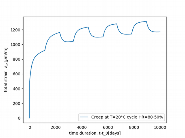
This test is available here.
The T-H-M loading is as follow:
@ExternalStateVariable "Temperature" 20.;
@ImposedStress "SXX" {0.0: 0, 8.64000000e+08: 0};
@ExternalStateVariable "SECH" {0.0: 1.0, 8.64000000e+08: 0.5};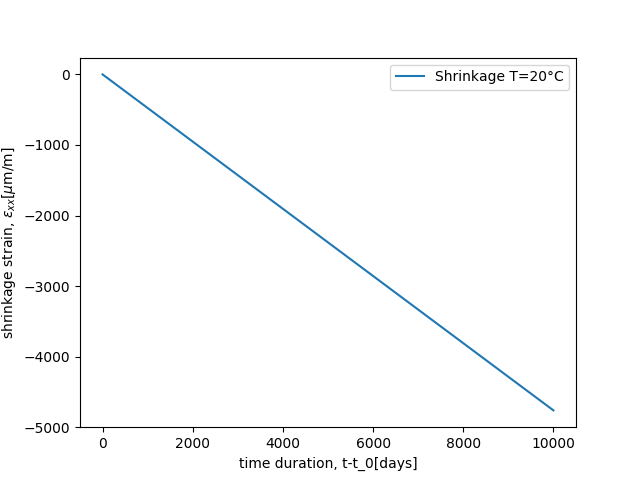
code_aster test cases:The same material properties as previously are used. For test cases
with drying, the GRANGER model with the parameters below is
use to simulate drying before mechanical modelling with the
Burger_EDF_CIWAP_2021 constitutive law.
| GRANGER material Properties | Values | Units |
|---|---|---|
| \(A\) | 4.3e-13 | m2/s |
| \(B\) | 0.07 | - |
| \(\frac{Q}{R}\) | 4679 | K |
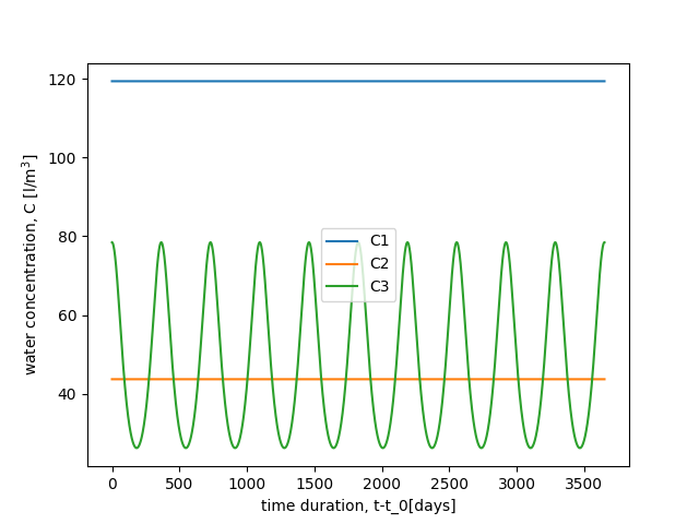
A desorption isotherm model is use to pass from humidity to water content and inversely. This desorption isotherm is not described here but is in the computation files. Firstly, the drying problem is solved in term of water content. Then, this water content evolution is converted into a relative humidity field by using desorption isotherm model.
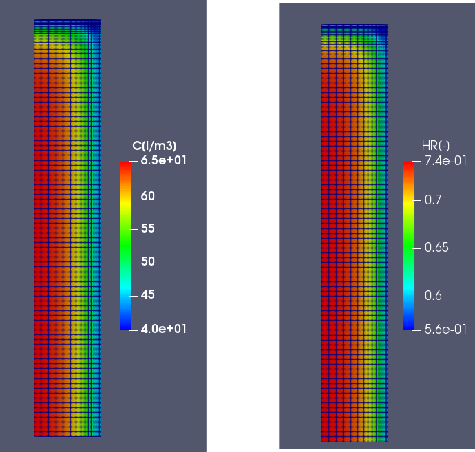
The water content of the three test cases below is presented here.
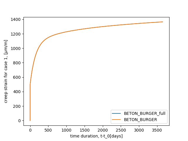
This test case concerns the modelling of uniaxial basic creep test on
16X100 cm specimen with 12 MPa of compression as proposed in [8]. A comparison between
BETON_BURGER and Burger_EDF_CIWAP_2021 is
shown below.
This test case concerns the modelling of uniaxial drying creep test
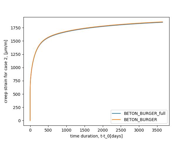
on 16X100 cm specimen with 12 MPa of compression as proposed in [8]. A comparison between
BETON_BURGER and Burger_EDF_CIWAP_2021 is
shown below.
This test case concerns the modelling of uniaxial drying creep test
on 16X100 cm specimen with 12 MPa of compression as proposed in [8] in case of drying-humidification
cycle condition. A comparison between BETON_BURGER and
Burger_EDF_CIWAP_2021 is shown below.