This tutorial shows how to implement in MFront mean-field homogenization schemes within the framework of 3d linear elasticity, for biphasic media.

These homogenization schemes are part of the namespace tfel::material::homogenization::elasticity. They are implemented via the DSL @MaterialLaw.

Available schemes

The implemented schemes for biphasic media are:

• Dilute scheme
• Mori-Tanaka scheme
• Voigt and Reuss bounds
• Isotropic Hashin-Shtrikman bounds

For dilute scheme and Mori-Tanaka scheme, the following assumptions are made:

• the microstructure is biphasic
• the phases are isotropic
• one phase is a matrix, the other is made by inclusions
• the shape of inclusions can be spherical, spheroidal, ellipsoidal, otherwise the mean strain localisator (for a single inclusion problem) can be provided by the user
• for non-spherical inclusions, we consider 3 possibilities of orientation distribution: isotropic, transverse isotropic and oriented

For Voigt, Reuss and Hashin-Shtrikman bounds, the following assumptions are made:

• N phases can be considered
• the phases can be anisotropic for Voigt and Reuss bounds, but only isotropic for Hashin-Shtrikman bounds

Example 1: a distribution of spherical inclusions

We begin with a basic example: a particulate composite with spherical inclusions.

Implementation in MFront

Here is the header of the mfront file:

@DSL MaterialLaw;
@Law Spherical;
@Material biphasic;
@UseQt true;

Here we want to let the user choose which scheme he wants to use: dilute scheme, Mori-Tanaka scheme… Hence, a real parameter is defined as an input, which can be 0 for dilute scheme, 1 for Mori-Tanaka… (f is the volume fraction of inclusion phase).

@StateVariable real scheme;
scheme.setEntryName("HomogenizationScheme");
@StateVariable stress E0;
E0.setEntryName("MatrixYoungModulus");
@StateVariable real nu0;
nu0.setEntryName("MatrixPoissonRatio");
@StateVariable stress Ei;
Ei.setEntryName("InclusionYoungModulus");
@StateVariable real nui;
nui.setEntryName("InclusionPoissonRatio");
@StateVariable real f;
f.setEntryName("InclusionVolumeFraction");

It is important not to forget the header files that must be included:

@TFELLibraries {"Material"};

@Includes{
#include "TFEL/Material/LinearHomogenizationSchemes.hxx"
#include "TFEL/Material/LinearHomogenizationBounds.hxx"
}

Note that @TFELLibraries lets the user specify a TFEL library to link with. The header LinearHomogenizationSchemes.hxx is needed for dilute scheme and Mori-Tanaka scheme, whereas here LinearHomogenizationBounds.hxx will be used for computing upper Hashin-Shtrikman (HS) bound. It is indeed known that the lower Hashin-Shtrikman bound is equal to the Mori-Tanaka scheme with spheres.

We choose the Young homogenized modulus E to be the output of our Function.

@Output stress E;

Here is the implementation of the different homogenized schemes:

@Function{
using namespace tfel::material::homogenization::elasticity;
std::pair<stress,real> pa;
if (scheme==real(0)){
pa=computeSphereDiluteScheme<real,stress>(E0,nu0,f,Ei,nui);
}
if (scheme==real(1)){
pa=computeSphereMoriTanakaScheme<real,stress>(E0,nu0,f,Ei,nui);
};
if (scheme==real(2)){
std::array<real,2> tab_f={1-f,f};
auto k0=E0/3/(1-2*nu0);
auto ki=Ei/3/(1-2*nui);
std::array<stress,2> tab_k={k0,ki};
auto mu0=E0/2/(1+nu0);
auto mui=Ei/2/(1+nui);
std::array<stress,2> tab_mu={mu0,mui};
auto pa2=computeIsotropicHashinShtrikmanBounds<3u,2u,real,stress>(tab_f,tab_k,tab_mu);
auto UB=std::get<1>(pa2);
auto kh=std::get<0>(UB);
auto muh=std::get<1>(UB);
auto Eh=9*kh*muh/(muh+3*kh);
auto nuh=(3*kh-2*muh)/2/(3*kh+muh);
pa={Eh,nuh};
};
E=std::get<0>(pa);
}

Hence, pa is a std::pair that returns the Young homogenized modulus and the homogenized Poisson ratio. The computation of dilute scheme and Mori-Tanaka scheme are straightforward.

The function computeIsotropicHashinShtrikmanBounds necessitates to give the arrays of volume fractions tab_f, bulk moduli tab_k and shear moduli tab_mu. The function returns a pair of pair. The first pair is lower HS bound, the second is upper HS bound (that we want here). Each bound is a pair whose first element is the bulk modulus, and whose second element is the shear modulus. The function is also available for plain strain elasticity (the first template argument is the dimension).

Results

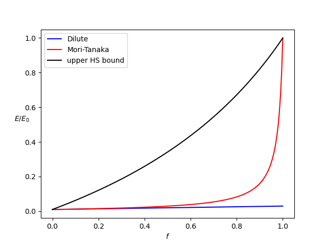
We choose interface python to compute the schemes for a volume fraction of spheres which goes from 0 to 1.

Here is the python file :

import src.biphasic as bip
from matplotlib import pyplot as plt
import numpy as np

frac=np.linspace(0,1,200)
E_DS=np.array([bip.biphasic_Spherical(0,1e9,0.2,100e9,0.3,f)/1e11 for f in frac])
E_MT=np.array([bip.biphasic_Spherical(1,1e9,0.2,100e9,0.3,f)/1e11 for f in frac])
E_HS=np.array([bip.biphasic_Spherical(2,1e9,0.2,100e9,0.3,f)/1e11 for f in frac])
plt.figure()
g1,=plt.plot(frac,E_DS,color="blue")
g2,=plt.plot(frac,E_MT,color="red")
g3,=plt.plot(frac,E_HS,color="black")
plt.legend([g1,g2,g3],['Dilute','Mori-Tanaka','upper HS bound'])
plt.xlabel(r'$f$')
plt.ylabel(r'$E/E_0$',rotation='horizontal')
plt.show()
plt.close()

The results are given by the following figure.

Example 2: distributions of ellipsoidal inclusions

The example of a composite with ellipsoidal inclusions can be implemented considering various examples of distributions. We will focus on Mori-Tanaka scheme, but dilute scheme can also be computed.

Implementation in MFront

The first lines are not so different from example 1, except the fact that we now define a real parameter distrib to let the user choose the distribution of ellipsoids: isotropic, transverse isotropic, or oriented. We also introduce the semi-lengths a,b,c of the ellipsoid.

@StateVariable real distrib;
distrib.setEntryName("TypeOfDistribution");
@StateVariable stress E0;
E0.setEntryName("MatrixYoungModulus");
@StateVariable real nu0;
nu0.setEntryName("MatrixPoissonRatio");
@StateVariable stress Ei;
Ei.setEntryName("InclusionYoungModulus");
@StateVariable real nui;
nui.setEntryName("InclusionPoissonRatio");
@StateVariable real f;
f.setEntryName("InclusionVolumeFraction");
@StateVariable length a;
a.setEntryName("FirstSemiLength");
@StateVariable length b;
b.setEntryName("SecondSemiLength");
@StateVariable length c;
c.setEntryName("ThirdSemiLength");

Note that the orientation for the oriented case will be fixed in the mfront file, and it will be the same for the transverse isotropic case which necessitates to gives the direction of one of the axes of the ellipsoid. But those orientations could also be inputs of the law.

Here is the Function block:

@Function{
tfel::math::tvector<3u,real> n_a={1,0,0};
tfel::math::tvector<3u,real> n_b={0,1,0};
using namespace tfel::material::homogenization::elasticity;
if (distrib==real(0)){
auto pa = computeIsotropicMoriTanakaScheme<real,stress,length>(E0,nu0,f,Ei,nui,a,b,c);
E1=std::get<0>(pa);
}
if (distrib==real(1)){
auto Chom=computeTransverseIsotropicMoriTanakaScheme<real,stress,length>(E0,nu0,f,Ei,nui,n_a,a,b,c);
auto Shom=invert(Chom);
E1=1/Shom(0,0);
}
if (distrib==real(2)){
auto Chom=computeOrientedMoriTanakaScheme<real,stress,length>(E0,nu0,f,Ei,nui,n_a,a,n_b,b,c);
auto Shom=invert(Chom);
E1=1/Shom(0,0);
}
}

For computeTransverseIsotropicMoriTanakaScheme, only one vector n_a is used. It specifies the direction of transverse isotropy. The ellipsoid has one axis aligned with this vector, and the semi-length of this axis is specified immediately after n_a (here a). This is in fact a special case of transverse isotropy for which the ellipsoid rotates around one of its principal axes. For computeOrientedMoriTanakaScheme, the first vector n_a is the direction of one axis, whose semi-length is precised immediately after (here a) and the same goes for the second vector and second semi-length. If the vectors are not normals, an error is returned. However, the norms of these vectors can be different from 1.

Results

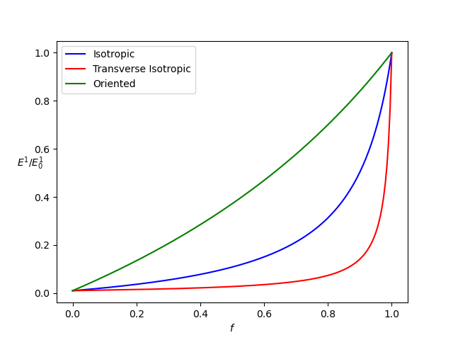
We choose interface python to compute the schemes for a volume fraction of ellipsoids which goes from 0 to 1.

Here is the python file :

import src.biphasic as bip
from matplotlib import pyplot as plt
import numpy as np


frac=np.linspace(0,1,200)
E_I=np.array([bip.biphasic_Ellipsoidal(0,1e9,0.2,100e9,0.3,f,30,1,1)/1e11 for f in frac])
E_TI=np.array([bip.biphasic_Ellipsoidal(1,1e9,0.2,100e9,0.3,f,1,30,1)/1e11 for f in frac])
E_O=np.array([bip.biphasic_Ellipsoidal(2,1e9,0.2,100e9,0.3,f,30,1,1)/1e11 for f in frac])
plt.figure()
g1,=plt.plot(frac,E_I,color="blue")
g2,=plt.plot(frac,E_TI,color="red")
g3,=plt.plot(frac,E_O,color="green")
plt.legend([g1,g2,g3],['Isotropic','Transverse Isotropic','Oriented'])
plt.xlabel(r'$f$')
plt.ylabel(r'$E^{1}/E^{1}_0$',rotation='horizontal')
plt.show()
plt.close()

We see here that we chose prolate spheroids for the ellipsoids, with aspect ratio of 30. The first case is the isotropic distribution, the second case is the transverse isotropic distribution where the biggest axis rotates in the y-z plane, and in the last case, the biggest axis is oriented in the x direction. The results are given by the following figure.