
The Cambridge (Cam) clay model describes the stress-dependent deformation behaviour of cohesive soils. Thereby, effects like
can be considered. Typical applications for the Cam clay model are
the calculation of soil strata, for example in geomechanical
simulations. The goal of this technical report is a consistent and clear
presentation of the basic modified Cam clay model ready for
implementation and practical use in continuum mechanical simulations
using FEM. Here, the material model interface MFront is
used. For the sake of compactness, a symbolic tensor notation is used
where the number of underscores indicates the order of the tensor
object.
In the small-strain setting there is an additive split of the linear strain tensor reading \[ \underline{\varepsilon }= \underline{\varepsilon}_\text{e}+ \underline{\varepsilon}_\text{p}\ . \]
The generalized Hooke’s law relates elastic strains with stresses as \[ \underline{\sigma }= \underline{\underline{D}}\,\colon\,\underline{\varepsilon}_\text{e}\ . \]
Splitting the stress tensor with respect to deviatoric and volumetric parts yields
\[ \underline{\sigma }= \underline{\sigma}^\text{D}+ \frac{1}{3}I_1(\underline{\sigma})\underline{I} \ . \] Therewith, the von-Mises stress and the hydrostatic pressure is defined as \[ q \coloneqq \sqrt{\dfrac{3}{2}\ \underline{\sigma}^\text{D}\,\colon\,\underline{\sigma}^\text{D}} \quad,\quad p \coloneqq -\frac{1}{3}I_1(\underline{\sigma}) \ . \] Consequently, positive values of \(p\) represent a pressure whereas negative values represent hydrostatic tension, as expected. With this, the stress tensor split reads \(\underline{\sigma }= \underline{\sigma}^\text{D}- p\underline{I}\). Later the following derivatives will be required: \[ \frac{\partial q}{\partial \underline{\sigma}} = \frac{3}{2}\ \frac{\underline{\sigma}^\text{D}}{q}\quad,\quad \frac{\partial p}{\partial \underline{\sigma}} = -\frac{1}{3}\ \underline{I} \ . \] Dealing with porous media there is a kinematic relation between porosity and volumetric strain. Let the total volume of an REV be divided into a pore volume and the solid volume: \[ V = V_{\text{S}} + V_{\text{P}} \ . \] Now, the porosity is defined as the pore volume fraction, i.,e. \(\phi=V_{\text{P}}/V\). Evaluating the mass balance equation of the porous solid yields the porosity evolution in the form \[\label{eq:porEvolution} \dot{\phi} - \phi\mathrm{div}(\dot{\vec{u}}) = \mathrm{tr}(\dot{\underline{\varepsilon}}) \ . \] Exploiting \(\mathrm{div}(\dot{\vec{u}})\equiv \mathrm{tr}(\dot{\underline{\varepsilon}})\) and separating the variables, this differential equation can be solved in a straightforward manner (cf. App.).
If the elastic volume changes are small compared to the plastic ones, the porosity (evolution) can be calculated from \(\varepsilon^\text{V}_\text{p}\) only. Instead of the porosity \(\phi\), the pore number \(e=V_{\text{P}} / V_{\text{S}}\) can equally be used with the relations
\[\label{eq:e-phiRelation} e = \frac{\phi}{1-\phi} \quad\text{with}\quad 1+e = (1-\phi)^{-1}\ . \]
The following set of equations fully describes the basic modified Cam clay model. Elasticity is
\[\label{eq:linearElasticity} \underline{\sigma }= \underline{\underline{D}}\,\colon\,\left(\underline{\varepsilon }- \underline{\varepsilon}_\text{p}\right) \ . \]
Then, the Cam clay yield function with the parameters \(M\) and \(p_\text{c}(e)\) is given by
\[ f \coloneqq q^2 + M p(p-p_\text{c}) \leq 0 \ . \]
An associated flow rule (normality rule) is used to obtain the plastic flow as
\[\label{eq:flowRule} \dot{\underline{\varepsilon}}_\text{p}= \dot{\varLambda}_\text{p}\ \underline{n} \quad\text{with}\quad \underline{n} =\frac{\underline{m}}{\|\underline{m}\|} \quad,\quad \underline{m} = \frac{\partial f}{\partial \underline{\sigma}} \ . \]
where \(\dot{\varLambda}_\text{p}\) denotes the plastic multiplier such that \(\text{d}{\varLambda}_\text{p}\) is the plastic increment and \(\underline{n}\) gives the direction of the plastic flow. The plastic volume change rate is obtained from:
\[ \dot{\varepsilon}_\text{p}^\text{V} = \mathrm{tr}(\dot{\underline{\varepsilon}}_\text{p}) = \dot{\varLambda}_\text{p}\,\mathrm{tr}(\underline{n})\ . %\tensor{I}\ppkt\tensor{n} \]
The so-called pre-consolidation pressure \(p_\text{c}\) represents the yield stress under isotropic compression and evolves as:
\[\label{eq:evolutionPc} \dot{p}_\text{c}= -\dot{\varepsilon}_\text{p}^\text{V} \vartheta(e)\ p_\text{c}\quad\text{with}\quad p_\text{c}\big{|}_{t=0} = p_{\text{c}0} \ . \]
This way, the pre-consolidation pressure increases in case of plastic compaction, i.,e. \(\dot{\varepsilon}_\text{p}^\text{V}<0\). Moreover, the pre-consolidation pressure remains constant during purely elastic loading. Furthermore, the parameter \(\vartheta\) depends on the pore number \(e\) or the porosity \(\phi\), respectively:
\[ \vartheta(e) = \frac{1+e}{\lambda - \kappa} = \frac{1}{(\lambda - \kappa)(1 - \phi)} = \vartheta(\phi) \ , \]
where the material constants \(\lambda, \kappa\) represent the slope of the virgin normal consolidation line and the normal swelling line, respectively (with \(\lambda>\kappa\)), in a semi-logarithmic \((1+e)-\ln p\) plot. This gives:
\[ \dot{p}_\text{c}= -\dot{\varepsilon}_\text{p}^\text{V} \left(\frac{1+e}{\lambda - \kappa}\right)\ p_\text{c}\ . \]
With the porosity evolution given by formula \(\eqref{eq:porEvolution}\), the system of constitutive equations for the modified Cam clay model is closed. This way, all the basic effects \(1.-5.\) are captured.
In order to refine effect \(5.\), namely load-path dependent elastic stiffness, an evolution equation for the hydrostatic pressure and the elastic volumetric strain, respectively, has to be added [1]:
\[\label{eq:evolutionP} \dot{p} = -\dot{\varepsilon}_\text{e}^\text{V} \left(\frac{1+e}{\kappa}\right)\ p \ . \]
As a consequence, the compression modulus becomes load-path-dependent, too. Then, care must be taken that the constitutive equations are still thermodynamically consistent [2]. I also seems counter-intuitive that the bulk modulus should increase with the pore number. For these reasons and for the sake of simplicity, linear elasticity is used here. This means instead of \(\eqref{eq:evolutionP}\) holds
\[\label{eq:constK} \dot{p} = -\dot{\varepsilon}_\text{e}^\text{V}\ K \ , \]
which is automatically fulfilled applying linear elasticity \(\eqref{eq:linearElasticity}\) with a constant bulk modulus \(K\).
For a time integration, the total values at the next instant of time are calculated from the current values and the increments, i.,e.
\[ \begin{align} \underline{\varepsilon}_\text{e}&\coloneqq {}^{k+1}\underline{\varepsilon}_\text{e}= {}^{k}\underline{\varepsilon}_\text{e}+ \theta\varDelta \underline{\varepsilon}_\text{e}\ , \\ \varLambda_p &\coloneqq {}^{k+1}\varLambda_p = {}^{k}\varLambda_p + \theta\varDelta \varLambda_p\ , \\ p_\text{c}&\coloneqq {}^{k+1}p_\text{c}= {}^{k}p_\text{c}+ \theta\varDelta p_\text{c}\ , \\ \phi &\coloneqq {}^{k+1}\phi = {}^{k}\phi + \theta\varDelta\phi \ , \end{align} \]
The discretized incremental evolution equation now read \[ \begin{align} \varDelta\underline{\varepsilon}_\text{p}&= \varDelta{\varLambda}_\text{p}\ \underline{n}\ , \\ \varDelta{\varepsilon}_\text{p}^\text{V} &= \varDelta{\varLambda}_\text{p}\,\mathrm{tr}(\underline{n})\ , \\ \varDelta{p}_\text{c}&= -\varDelta{\varepsilon}_\text{p}^\text{V} \vartheta(e)\ p_\text{c}\ , \\ \varDelta\phi &= (1-\phi) \varDelta\varepsilon^\text{V} \ . \end{align} \]
With this, the discretized set of equations has the form
\[\label{eq:incrementalSystem} \begin{align} \underline{f}_{\!\varepsilon_\text{e}} &= \varDelta\underline{\varepsilon}_\text{e}+ \varDelta\varLambda_p\ \underline{n} - \varDelta\underline{\varepsilon }= \underline{0} \ ,\\ f_{\!\varLambda_p} &= q^2 + M^2(p^2 - p\,p_\text{c}) = 0 \ , \label{eq:flp}\\ %\dfrac{1}{E^2} f_{p_\text{c}} &= \varDelta p_\text{c}+ \varDelta\varepsilon_\text{p}^\text{V} \vartheta(\phi)\ p_\text{c}= 0 \ , \label{eq:fpc} \\ f_{\phi} &= \varDelta\phi - (1-\phi) \varDelta\varepsilon^\text{V} = 0 \ , \label{eq:fphi} \end{align} \]
where the total values are the values at the next instant of time, meaning \(q={}^{k+1}q, p={}^{k+1}p\). For the partial derivatives the functional dependencies are required. They read
\[\label{eq:functionalDependence} \begin{align} \underline{f}_{\!\varepsilon_\text{e}} &= \underline{\underline{D}}_{\!\varepsilon_\text{e}}(\varDelta\underline{\varepsilon}_\text{e}, \varDelta\varLambda_p, \varDelta p_\text{c}) \ ,\\ f_{\!\varLambda_p} &= f_{\varLambda_p}(\varDelta\underline{\varepsilon}_\text{e}, \varDelta p_\text{c}) \ , \\ f_{p_\text{c}} &= f_{p_\text{c}}(\varDelta\underline{\varepsilon}_\text{e}, \varDelta\varLambda_p, \varDelta p_\text{c}, \varDelta\phi)\ , \\ f_{\phi} &= f_{\phi}(\varDelta\phi) \ , \end{align} \]
where it was taken into account, that \(q(\underline{\sigma}), p(\underline{\sigma})\) and \(\underline{\sigma}(\varDelta\underline{\varepsilon}_\text{e})\) and \(\underline{n}(q, p, p_\text{c})\) and \(\varDelta\varepsilon_\text{p}^\text{V}(\varDelta\varLambda_p, \underline{n})\).
For the solution of the incremental set of equations \(\eqref{eq:incrementalSystem}\) with the Newton-Raphson method the partial derivatives with respect to the increments of the unknowns are required. They read
\[\label{eqset:partialDerivatives} \begin{align} \frac{\partial\underline{f}_{\!\varepsilon_\text{e}}}{\partial\varDelta\underline{\varepsilon}_\text{e}} &= \underline{\underline{I}} + \varDelta\varLambda_p\frac{\partial\underline{n}}{\partial\varDelta\underline{\varepsilon}_\text{e}} \quad\text{with}\quad \underline{\underline{I}}=\vec{e}_a\,\otimes\,\vec{e}_b\,\otimes\,\vec{e}_a\,\otimes\,\vec{e}_b \ , \\ \frac{\partial\underline{f}_{\!\varepsilon_\text{e}}}{\partial\varDelta\varLambda_p} &= \underline{n}\ , \\ \frac{\partial\underline{f}_{\!\varepsilon_\text{e}}}{\partial\varDelta p_\text{c}} &= \varDelta\varLambda_p \ \frac{\partial\underline{n}}{\partial\varDelta p_\text{c}} , \\[2mm] \frac{\partial f_{\!\varLambda_p}}{\partial\varDelta\underline{\varepsilon}_\text{e}} &= \frac{\partial f_{\!\varLambda_p}}{\partial \underline{\sigma}} : \frac{\partial \underline{\sigma}}{\partial \underline{\varepsilon}_\text{e}} : \frac{\partial\underline{\varepsilon}_\text{e}}{\partial\varDelta\underline{\varepsilon}_\text{e}} = \underline{m} : \underline{\underline{D}}\ \theta\ , %: \theta\tensorf{I} \\ \frac{\partial f_{\!\varLambda_p}}{\partial\varDelta p_\text{c}} &= \frac{f_{\!\varLambda_p}}{\partial p_\text{c}}\ \frac{\partial p_\text{c}}{\partial \varDelta p_\text{c}} = -p M^2\, \theta\ , \\[2mm] \frac{\partial f_{p_\text{c}}}{\partial\varDelta\underline{\varepsilon}_\text{e}} &= \frac{\partial f_{p_\text{c}}}{\partial\underline{n}} : \frac{\partial\underline{n}}{\partial\varDelta\underline{\varepsilon}_\text{e}}\ , \\ \frac{\partial f_{p_\text{c}}}{\partial\varDelta\varLambda_p} &= \frac{\partial f_{p_\text{c}}}{\partial\varDelta\varepsilon_\text{p}^\text{V}}\ \frac{\partial\varDelta\varepsilon_\text{p}^\text{V}}{\partial\varLambda_p} = \vartheta p_\text{c}\,\mathrm{tr}(\underline{n})\ , \\ \frac{\partial f_{p_\text{c}}}{\partial\varDelta p_\text{c}} &= 1 + \vartheta\varDelta\varepsilon_\text{p}^\text{V}\theta + \frac{\partial f_{p_\text{c}}}{\partial\underline{n}} : \frac{\partial\underline{n}}{\partial\varDelta p_\text{c}}\ , \\ \frac{\partial f_{p_\text{c}}}{\partial\varDelta\phi} &= \varDelta\varepsilon_\text{p}^\text{V} p_\text{c}\frac{\partial\vartheta(\phi)}{\partial\phi}\ \frac{\partial\phi}{\partial\varDelta\phi} = \frac{\varDelta\varepsilon_\text{p}^\text{V} p_\text{c}\,\theta }{(\lambda - \kappa)(1 - \phi)^2}\ , = \frac{\varDelta\varepsilon_\text{p}^\text{V} p_\text{c}\,\vartheta\,\theta }{(1 - \phi)}\ , \\[2mm] \frac{\partial f_{\phi}}{\partial\varDelta\phi} &= 1 + \theta\varDelta\varepsilon^\text{V} \ . \end{align} \]
All other partial derivatives vanish according to the (missing) dependencies \(\eqref{eq:functionalDependence}\). Using the normalized flow direction \(\underline{n}\), the derivatives with respect to some variable \(X\) can be obtained with the following rule:
\[\begin{align} \frac{\partial\underline{n}}{\partial X} = \frac{1}{m}\left\{\frac{\partial\underline{m}}{\partial X} - \frac{1}{2}\,\underline{n}\,\otimes\,\frac{1}{m}\frac{\partial m^2}{\partial X} \right\}\quad\text{with}\quad m=\|\underline{m}\| \ . \end{align}\]
Now, the missing expressions in overview \(\eqref{eqset:partialDerivatives}\) can be calculated as
\[\begin{align} \underline{m} &= \frac{\partial f}{\partial \underline{\sigma}} = \frac{\partial f}{\partial q}\,\frac{\partial q}{\partial \underline{\sigma}} +\frac{\partial f}{\partial p}\,\frac{\partial p}{\partial \underline{\sigma}} = 3\underline{\sigma}^\text{D}- \dfrac{M^2}{3}(2p-p_\text{c}) \underline{I} \ , \\ m^2 &= \underline{m} : \underline{m} = 6q^2 + \dfrac{M^4}{3}(2p-p_\text{c})^2 \qquad , \quad \underline{n} = \underline{m}/m \ , \\ \frac{\partial\underline{m}}{\partial\underline{\varepsilon}_\text{e}} &= \left\{ \frac{\partial\underline{m}}{\partial q}\,\frac{\partial q}{\partial \underline{\sigma}} + \frac{\partial\underline{m}}{\partial p}\,\frac{\partial p}{\partial \underline{\sigma}} \right\} : \frac{\partial \underline{\sigma}}{\partial \underline{\varepsilon}_\text{e}} = \left\{ 3\underline{\underline{P}} + \dfrac{2}{9} M^2 \underline{I}\,\otimes\,\underline{I} \right\} : \underline{\underline{D}} \ , \\ \frac{\partial m^2}{\partial\underline{\varepsilon}_\text{e}} &= \left\{ \frac{\partial m^2}{\partial q}\,\frac{\partial q}{\partial \underline{\sigma}} +\frac{\partial m^2}{\partial p}\,\frac{\partial p}{\partial \underline{\sigma}} \right\} : \frac{\partial \underline{\sigma}}{\partial \underline{\varepsilon}_\text{e}} = \left\{ 18\underline{\sigma}^\text{D}- \dfrac{4}{9} M^4 (2p-p_\text{c})\underline{I} \right\} : \underline{\underline{D}} \ , \\ \frac{\partial\underline{n}}{\partial\varDelta\underline{\varepsilon}_\text{e}} &= \frac{1}{m}\left\{\frac{\partial\underline{m}}{\partial\underline{\varepsilon}_\text{e}} - \frac{1}{2}\,\underline{n}\,\otimes\,\frac{1}{m}\frac{\partial m^2}{\partial\underline{\varepsilon}_\text{e}} \right\} : \frac{\partial\underline{\varepsilon}_\text{e}}{\partial\varDelta\underline{\varepsilon}_\text{e}} \ , \\ \frac{\partial\underline{n}}{\partial\varDelta p_\text{c}} &= \frac{1}{m}\left\{\frac{\partial\underline{m}}{\partial p_\text{c}} - \frac{1}{2}\,\underline{n}\,\otimes\,\frac{1}{m}\frac{\partial m^2}{\partial p_\text{c}} \right\} \frac{\partial p_\text{c}}{\partial\varDelta p_\text{c}} = \frac{M^2}{3m}\left\{\underline{I} + M^2(2p-p_\text{c})\,\underline{n}/m \right\} \theta\ , \\ \frac{\partial f_{p_\text{c}}}{\partial\underline{n}} &= \frac{f_{p_\text{c}}}{\partial\varDelta\varepsilon_\text{p}^\text{V}}\, \frac{\partial\varDelta\varepsilon_\text{p}^\text{V}}{\partial\underline{n}} = p_\text{c}\vartheta\ \varDelta\varLambda_p \underline{I} \ . \end{align}\]
The solution of System \(\eqref{eq:incrementalSystem}\) can be accomplished based on the Karush Kuhn Tucker conditions with an elastic predictor and a plastic corrector step. This leads to a radial return mapping algorithm (also known as active set search). Alternatively, the case distinction can be avoided using the Fischer-Burmeister complementary condition [3, 4]. Both methods can be used in MFront [5, 6].
It is recommended to normalize all residuals \(\eqref{eq:incrementalSystem}\) to some similar order of magnitude, e.,g. as strains. For this, equation \(\eqref{eq:flp}\) can be divided by some characteristic value:
\[\begin{align} f_{\!\varLambda_p} &= f / \hat{f} = \left\{q^2 + M^2(p^2 - p\,p_\text{c})\right\} / (E\,p_{\text{c}0}) \ . %f_{p_\c} &= \left\{ \varDelta p_\c + \varDelta\varepsilon_\p^\text{V} \vartheta(\phi)\ p_\c \right\} / E \end{align}\]
Here \(\hat{f} = E\,p_{\text{c}0}\) was chosen with the elastic modulus and the initial value of the pre-consolidation pressure. Of course, this has to be considered in the corresponding partial derivatives {(\(\ref{eqset:partialDerivatives}\)d–f)}.
Instead of applying the same procedure to \(f_{p_\text{c}}\) it is advantageous to directly normalize the corresponding independent variable \(p_\text{c}\). Then, the new reduced integration variable is
\[ p_\text{c}^r\coloneqq p_\text{c}/ \hat{p}_\text{c}= p_\text{c}/ p_{\text{c}0} \ . \]
Thus, the partial derivatives with respect to \(p_\text{c}\) have to be replaced as
\[ \frac{\partial (\ast)}{\partial p_\text{c}} \rightarrow \frac{\partial (\ast)}{\partial p_\text{c}^r} = \frac{1}{\hat{p}_\text{c}} \frac{\partial (\ast)}{\partial p_\text{c}} \ . \]
Consequently, all integration variables $_, p, p^r, $ are dimensionless, strain-like variables, which improves the condition number of the set of equations.
In order to stabilize the numerical behaviour two more minor modifications are beneficial. The first one regards some (initial) state with zero stress. Then \(f=0\) is indicating potential plastic loading, but plastic flow \(\eqref{eq:flowRule}\) is undetermined. To prevent this case, a small (ambient) pressure \(p_\text{amb}\) can be added to the hydrostatic pressure, i.,e.
\[ p \coloneqq -I_1(\underline{\sigma})/3 + p_\text{amb} \ . \]
Hence, a small initial elastic range is provided.
Another problem occurs in case of strong softening and dilatancy: \(p_\text{c}\rightarrow 0\) and the yield surface contracts until it degenerates to a single point such that the direction of plastic flow is undefined. In order to limit the decrease of \(p_\text{c}\) to some minimal pre-consolidation pressure \(p^\text{min}_\text{c}\) the evolution equation \(\eqref{eq:evolutionPc}\) is modified to
\[\label{eq:pcMin} \dot{p}_\text{c}= -\dot{\varepsilon}_\text{p}^\text{V} \vartheta(e)\ (p_\text{c}- p^\text{min}_\text{c}) \quad\text{with}\quad p_\text{c}\big{|}_{t=0} = p_{\text{c}0} \ , \]
where the normalization from above can be applied again. A reasonably small value for \(p^\text{min}_\text{c}\) can be, e.,g., the ambient atmospheric pressure. The modifications need to be considered in Eq.~\(\eqref{eq:fpc}\) and its derivatives.
The number of equations in System \(\eqref{eq:incrementalSystem}\) can be reduced exploiting the minor influence of the porosity in a given time step. Since \(\phi\) usually does not significantly change during the strain increment, it can be updated explicitly at the end of the time step [7]. Exploiting formula \(\eqref{eq:evolutionPhi}\) yields
\[\begin{align} {}^{k+1}\!\phi &= 1 -\, (1-{}^{k}\!\phi) \exp(-\Delta\varepsilon^\text{V}) \quad\text{or}\\ {}^{k+1}\!\phi &= {}^{k}\!\phi + \Delta\phi \quad\text{with}\quad \Delta\phi = (1-{}^{k}\!\phi) \left[ 1- \exp(-\Delta\varepsilon^\text{V}) \right]\ . \end{align}\]
Thus, the residual equation \(\eqref{eq:fphi}\) and the corresponding derivatives can be omitted. The pore number follows directly from the new porosity value using the relation
\[ 1 + \,{}^{k+1}\!e = \frac{1}{1-\, {}^{k+1}\!\phi} %\quad\with\quad 1-\phi = (1-{}^{0}\!\phi) \exp(\minus\varepsilon^\text{V}) \ . \]
MFrontFor the MFront implementation the domain specific
language (DSL) Implicit was used, cf. [5, 8]. The coupling
to OpenGeoSys [9, 10] is done using MGIS
[6]. The
implementation is part of the OpenGeoSys source code,
cf. https://gitlab.opengeosys.org.
In the preamble of the MFront code the parameters are
specified and integration variables are declared. Note that a is a
persistent variable and an integration variable, whereas an is also
persistent but no integration variable.
// environmental parameters (default values)
@Parameter stress pamb = 1e+3; //Pa
@PhysicalBounds pamb in [0:*[;
pamb.setEntryName("AmbientPressure");

// material parameters
@MaterialProperty stress young;
@PhysicalBounds young in [0:*[;
young.setGlossaryName("YoungModulus");
...
@StateVariable real lp;
lp.setGlossaryName("EquivalentPlasticStrain");
@IntegrationVariable strain rpc;
@AuxiliaryStateVariable stress pc;
pc.setEntryName("PreConsolidationPressure");
@AuxiliaryStateVariable real phi;
phi.setGlossaryName("Porosity");
...
The semi-explicit solution scheme is then implemented with three basic steps:
@InitLocalVariables{
  //elastic predictor step
}
@Integrator{
  //plastic corrector step
}
@UpdateAuxiliaryStateVariables{
  //explicit porosity update
}MTestMFront provides the tool MTest for testing
the implemented material behaviour at a single material point
(integration point), see [5]. For this, non-monotonic loading
sequences can be prescribed in terms of stress and strain
trajectories.
In order to test the consolidation behaviour, plane strain simple shear tests were conducted with the same initial state but three different loading trajectories. To be precise, first the hydrostatic pressure \(p\) was increased until \(0.25\,p_{\text{c}0}, 0.5\,p_{\text{c}0}\) or \(0.75\,p_{\text{c}0}\). This results in the so-called overconsolidation ratios (OCR) of \(4, 2, 4/3\). From this hydrostatic stress state, shear is applied up to the strain \(\varepsilon_{xy}=0.01\).
| \(E\,(Pa)\) | \(\nu\) | \(M\) | \(\lambda\) | \(\kappa\) | \(\phi_0\) | \(p_\text{c}0\,(Pa)\) | \(p_{\text{amb}}\,(Pa)\) |
|---|---|---|---|---|---|---|---|
| \(150\cdot10^{9}\) | \(0.3\) | \(1.5\) | \(7.7\cdot10^{-3}\) | \(6.6\cdot10^{-4}\) | \(0.44\) | \(30\cdot10^{6}\) | \(0\cdot10^{3}\) |
The material parameters are given in Table 1. It should be noted that only the difference \(\lambda - \kappa\) plays a role in the basic model with elastic parameters. Considering the OCR, there are three different cases (cf. Figure 1):
For \(\text{OCR}>2\) the shearing is accompanied by a plastic expansion (dilatancy) with \(\varepsilon_\text{p}^\text{V}>0\), which causes softening until the critical state is reached.
For \(\text{OCR}=2\) shearing until yield leads directly to the critical state. Considering the state of the soil (porosity, stress, volume) this is a natural asymptotic state. Further shearing does not alter that state anymore. Hence, there is ideal plastic behaviour.
For \(\text{OCR}<2\) the shearing is accompanied by a plastic compaction (contractant flow, consolidation) with \(\varepsilon_\text{p}^\text{V}<0\), which causes hardening until the critical state is reached.
%TODO: OCR=1 means normally consolidated, OCR>1 describes an over-consolidated state %TODO: OCR=maximum pressure (=pre-consolidation pressure) / current pressure

The stress trajectories, and the final yield surfaces are illustrated in the \(p,q\)-space together with the initial yield surface and the critical state line (CSL).
Now, the same consolidated shear loading is applied, but there are two different initial states: a high value of the initial pre-consolidation pressure \(p_{\text{c}0}\) resembles a heavily pre-consolidated, compacted (dense) soil material, whereas a low value of \(p_{\text{c}0}\) resembles a loosened initial state.


As can be seen in Figures 3 and 4, the materials thrive to the same (asymptotic) critical state, since the CSL is identical. However, this is either accomplished by hardening (contraction) or softening (dilatancy).
OpenGeoSysAs a next step the shear test from the previous section was repeated
using OpenGeoSys, but without consolidation phase. A unit
square domain was meshed with only one finite element. At the boundaries
(top, bottom, left, right) Dirichlet boundary conditions~(BCs) were
prescribed. The top boundary was loaded by a linear ramp from time \(0\) to \(1\,\)s. The material parameters were taken
from Table 1 with only one difference: As the test has no
pre-consolidation phase, it is starting from zero stress and due to the
reasons explained in Section 3.2 some small initial ambient pressure
\(p_{\text{amb}}=1\cdot10^{3}\),Pa was
added.
| Test | BC left | BC right | BC top | BC bottom | behaviour |
|---|---|---|---|---|---|
| Shear \(xy\) | free | free | \(u_x=-0.05t\) | \(u_x=u_y=0\) | no convergence |
| Shear \(xy\) | free | free | \(u_x=-0.05t, u_y=0\) | \(u_x=u_y=0\) | convergence |

left) or free
(right).In order to have true simple shear the top BC \(u_y=0\) has to be applied. Else there is a tilting effect, and the deformation consists of shear and bending. As this is related to some parts with dominant tension stresses, convergence cannot be achieved with the Cam clay model (cf. next section). Note also that for pure shear \(\varepsilon^\text{V}=0\) and the volume and porosity thus remain constant. %(even for \(\varepsilon^\text{V}\neq 0\))
OpenGeoSysIt must be noted that the Cam clay model is primarily intended to capture the shear behaviour of soil materials cohesion. Hence, the uniaxial stress states with free boundaries cannot be sustained just as these states cannot be reached in reality. As an example, uniaxial tension causes pronounced lateral stretching due to plastic volume increase (dilatancy). The application of some minimal pre-consolidation pressure can help to stabilize the simulation, but convergence cannot be expected in general.
Still, the biaxial tension/compression behaviour can be simulated to a certain degree. The Table 3 shows under which conditions convergence can be expected. In the converged cases a homogeneous solution was obtained as expected.
| Test | BC left | BC right | BC top | BC bottom | convergence |
|---|---|---|---|---|---|
| Uniax. compr. \(y\) | \(u_x=0\) | free | \(u_y=-0.05t\) | \(u_y=0\) | no |
| Uniax. tension \(y\) | \(u_x=0\) | free | \(u_y=+0.05t\) | \(u_y=0\) | no |
| Biaxial compr. \(x,y\) | \(u_x=0\) | \(u_x=-0.05 t\) | \(u_y=-0.05t\) | \(u_y=0\) | yes |
| Biaxial tension \(x,y\) | \(u_x=0\) | \(u_x=+0.05 t\) | \(u_y=+0.05t\) | \(u_y=0\) | (yes) |
| Biaxial mixed \(x,y\) | \(u_x=0\) | \(u_x=+0.05 t\) | \(u_y=-0.05t\) | \(u_y=0\) | yes |
| Biaxial mixed \(x,y\) | \(u_x=0\) | \(u_x=-0.05 t\) | \(u_y=+0.05t\) | \(u_y=0\) | yes |
It is interesting to note that the biaxial tension test can be simulated with the Cam clay model. In order to achieve convergence the drop of the pre-consolidation pressure has to be limited. For this, either the value of the parameter difference \(\lambda - \kappa\) is increased or some minimal value \(p^\text{min}_\text{c}\) has to be ensured according to Eq.~\(\eqref{eq:pcMin}\).

As a benchmark to existing results an axially-symmetric triaxial compression test was performed. For this, a cylindrical domain of height \(100\),m and radius \(25\),m is meshed with \(100\times 25\) finite elements. At the left and bottom boundaries symmetry BCs of Dirichlet type are prescribed. The top and right boundaries are loaded by prescribing an axial and a confining pressure \(p_{\text{con}}\), respectively. The loading consists of two stages, similar to Section 5.1:
As the simulation time is irrelevant it is again set to \(1\,\)s. The material parameters are taken from .
| \(E (Pa)\) | \(\nu\) | \(M\) | \(\lambda\) | \(\kappa\) | \(\phi_0\) | $p_ (Pa) | \(p_{\text{amb}}\) (Pa)$ |
|---|---|---|---|---|---|---|---|
| \(52\cdot10^{6}\) | \(0.3\) | \(1.2\) | \(7.7\cdot10^{-2}\) | \(6.6\cdot10^{-3}\) | \(0.44\) | \(200\cdot10^{3}\) | \(1\cdot10^{3}\) |
The material and loading parameters were chosen such that the stress trajectory approaches the CSL from the right but does not meet it (cf. Figure 9). When this happens there will be zero resistance to plastic flow causing an infinite strain increment in the stress-controlled test and no convergence can be expected. The tendency can already be seen in Figure 8 with the steep increase of the equivalent plastic strain.

The curve of the pre-consolidation pressure (cf. Figure 8 top) shows monotonic hardening related to the plastic compaction (cf. Figure 8 bottom).

top, unit Pa) and strain measures
(bottom) at some arbitrary integration point.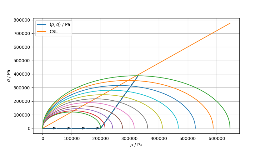
In order to check the accuracy of the numerical results, they were compared to an analytical solution [11] for proportional loading. For this, the straight stress path from \((q=0, p=p_{\text{con}})\) until the final state is considered (cf. Figure 9). The plot of the von-Mises stress over the corresponding equivalent strain defined by \(\varepsilon_{\text{q}}^2= {\tfrac{2}{3}\ \underline{\varepsilon}^\text{D}\,\colon\,\underline{\varepsilon}^\text{D}}\) shows accurate agreement between numerical and analytical solution (cf. also the appendix). Minor deviations might arise from the assumption \(\eqref{eq:evolutionP}\) [11], whereas a constant bulk modulus according to Eq. \(\eqref{eq:constK}\) was applied here. Considering the radial and circumferential strains another peculiarity is found (cf. Figure 10): The initial plastic compaction causes lateral (i.,e. radial and circumferential) contraction. However, with increasing axial compression this necessarily turns into expansion. Note also that for this test the magnitude of the strains is beyond the scope of the linear strain measure.

top) and a comparison between
analytical and numerical solution (bottom).As an alternative the test can, of course, also be conducted displacement-controlled. However, in doing so it was found that the homogeneous solution becomes unstable and strain localization occurs at the top of the domain. Apparently, at some integration points softening sets in even though the homogeneous solution only shows monotonic hardening. Varying the mesh size and topology, convergence could be achieved in some cases, indicating a strong mesh dependency.
The presented Cam clay material model has a simple structure, but can capture several characteristic phenomena of soil materials very well. However, it must be considered with caution when applied to realistic finite element simulations. The major limitations have two origins: first, the missing cohesion and second, the dilatant/softening part of the captured material behaviour. The provided numerical refinements can stabilize this only to a limited degree. It seems that the softening can cause a pronounced strain localization, which requires special strategies for regularization of the underlying ill-posed mathematical problem [12]. In order to include finite cohesion different modifications of the Cam clay model have been proposed [13]. Finally, mechanical loading in the vicinity of the critical state can easily cause large deformations, a finite strain formulation should be considered in the future [1, 2].
In order to check the convergence rate of the Cam clay implementation the consolidated shear test from Section~\(\ref{sec:mtestResults}\) was considered again. The parameters were taken from Table 1. The hydrostatic pressure \(p\) was increased until \(0.66\,p_{\text{c}0}\) resulting in an OCR of \(1.5\). From this hydrostatic stress state, shear is applied up to the strain \(\varepsilon_{xy}=5\cdot10^{-4}\) within \(20\) time steps.

MFront implementation
and MTest. Within the first \(12\) steps the behavior is purely elastic
(top), followed by contractant plastic flow
(bottom).As can be seen in Figure 11, convergence is achieved in one step in
the elastic stage (top). In the plastic stage
(bottom), the typical acceleration of convergence when
approaching the solution is observed (asymptotic quadratic convergence).
However, the convergence depends on the plastic flow behavior dictated
by the parameters \(M\), \(\lambda-\kappa\) and \(p_{\text{c}0}\) and can reduce to
super-linear (order \(\in [1,2]\)).
The implementation of the modified Cam clay model can be extended to
orthotropic elastic behavior using the so-called standard bricks within
MFront. Thus just one line of code need to be added:
@Brick StandardElasticity;
@OrthotropicBehaviour<Pipe>;
As a consequence the nine independent constants of orthotropic elasticity are already declared.
// material parameters
// Note: YoungModulus and PoissonRatio defined as parameters
// Note: Glossary names are already given; entry names are newly defined
@MaterialProperty real M;
@PhysicalBounds M in [0:*[;
M.setEntryName("CriticalStateLineSlope");
...
However, from the physical point of view it might be more realistic to consider the anisotropy both for the elastic and plastic behavior.
Given is the evolution equation for the porosity:
\[ \dot{\phi} - \phi\mathrm{div}(\dot{\vec{u}}) = \mathrm{tr}(\dot{\underline{\varepsilon}}) \quad\text{with}\quad \varepsilon^\text{V} = \mathrm{tr}({\underline{\varepsilon}}) \ . \]
Exploiting \(\mathrm{div}(\dot{\vec{u}})\equiv \mathrm{tr}(\dot{\underline{\varepsilon}})\) and separating the variables yields the form \[ \frac{\text{d}\phi}{1-\phi} = \text{d}\varepsilon^\text{V} \ . \] Integration over some time increment \(\varDelta t\) with \(\phi(t)={}^{k\!}\phi\) and \(\phi(t+\varDelta t)={}^{k+1\!}\phi\) as well as \(\Delta\varepsilon^\text{V}={}^{k+1\!}\varepsilon^\text{V}-{}^{k\!}\varepsilon^\text{V}\) as the volumetric strain increment, i.,e. \[ \int\limits_{{}^{k\!}\phi}^{{}^{k+1\!}\phi} \frac{\text{d}\phi}{1-\phi} = \int\limits_{{}^{k\!}\varepsilon^\text{V}}^{{}^{k+1\!}\varepsilon^\text{V}} \text{d}\varepsilon^\text{V} \ . \] then results in the incremental solution \[\label{eq:evolutionPhi} 1 -\, {}^{k+1}\!\phi = (1-{}^{k}\!\phi) \exp(-\Delta\varepsilon^\text{V}) \ . \] Integration over the whole process time span with the initial values \(\phi(t=0)={}^{0\!}\phi\) and \(\varepsilon^\text{V}(t=0)=0\) results in \[\label{eq:totalEvolutionPhi} 1-\phi = (1-{}^{0}\!\phi) \exp(-\varepsilon^\text{V}) \ . \] Combining \(\eqref{eq:totalEvolutionPhi}\) with \(\eqref{eq:evolutionPc}\) finally yields the evolution of the pre-consolidation pressure: \[ \dot{p}_\text{c}= -\frac{\dot{\varepsilon}_\text{p}^\text{V} p_\text{c}}{(\lambda - \kappa)(1-{}^{0}\!\phi) \exp(-\varepsilon^\text{V})} \ . \]
A straight stress path from \((p,q)=(0, p_{\text{c}0})\) until the final state \((p,q)=(387387, 330129)\ \)Pa is considered: \[ q = k\,(p-p_{\text{c}0}) \ . \]
The analytical solution [11] for the corresponding equivalent strain \(\varepsilon_{\text{q}}^2= {\tfrac{2}{3}\ \underline{\varepsilon}^\text{D}\,\colon\,\underline{\varepsilon}^\text{D}}\) reads
\[ \varepsilon_{\text{q}} = \varepsilon^\text{e}_{\text{q}} + \varepsilon^\text{p}_{\text{q}} \]
and to be precise, using the abbreviations \(C = (\lambda-\kappa)\) and \(\alpha = 3(1-2\nu) / (2(1+\nu))\) it is
\[\begin{align} (1+e_0)\,\varepsilon^\text{e}_{\text{q}} &= \ln\left[\left(1-\frac{q}{kp}\right)^{\frac{2Ck}{k^2-M^2}-\frac{\kappa k}{3\alpha}}\right]\ ,\\ (1+e_0)\,\varepsilon^\text{p}_{\text{q}} &= \ln\left[\left(1-\frac{q}{Mp}\right)^{\frac{Ck}{M(M-k)}} \cdot\left(1+\frac{q}{Mp}\right)^{\frac{Ck}{M(M+k)}}\right] - 2 \frac{C}{M}\arctan\left(\frac{q}{Mp}\right)\ . \end{align}\]