Benchmarks
Profiling tools
MFEM-MGIS provides a simple tool for profiling your application, consisting mainly in generating a time table of timed sections respecting the call stack (tree). The master or root timer of the call stack is initialized during the general initialization of mfem-mgis:
mfem_mgis::initialize(argc, argv);
Displaying the time table in your terminal is done by adding the following function call:
mfem_mgis::Profiler::timers::print_timers();
This is an example of an output:
MPI feature activated, rank 0:
|-- start timetable -------------------------------------------------------------------------------------------------------------------------------------------------------------------------------------|
|    name                                                                  |    number Of Calls |             min(s) |            mean(s) |             max(s) |            part(%) |             imb(%) |
|--------------------------------------------------------------------------------------------------------------------------------------------------------------------------------------------------------|
| > root                                                                   |                  1 |           0.061155 |           0.061313 |           0.061512 |        100.000000% |          0.003254% |
| |--> Solve                                                               |                  1 |           0.056359 |           0.056493 |           0.056539 |         91.914400% |          0.000812% |
|    |--> NonLinearEvolutionProblem::solve                                 |                  1 |           0.056359 |           0.056492 |           0.056538 |         91.913194% |          0.000812% |
|       |--> NonLinearEvolutionProblemImplementationBase::solve            |                  1 |           0.056357 |           0.056490 |           0.056536 |         91.909814% |          0.000810% |
|          |--> NewtonSolver::Mult                                         |                  1 |           0.056351 |           0.056483 |           0.056528 |         91.897665% |          0.000798% |
|             |--> NewtonSolver::computeNewtonCorrection                   |                 10 |           0.048653 |           0.048706 |           0.048851 |         79.416040% |          0.002969% |
|                |--> NewtonSolver::getJacobian                            |                 10 |           0.020212 |           0.020215 |           0.020220 |         32.870789% |          0.000239% |
|          |--> NonLinearEvolutionProblemImplementationBase::setup         |                  1 |           0.000004 |           0.000005 |           0.000006 |          0.009562% |          0.148211% |
| |--> FiniteElementDiscretization::constructor                            |                  1 |           0.002696 |           0.002717 |           0.002760 |          4.487192% |          0.015873% |
|    |--> loadMesh                                                         |                  1 |           0.000944 |           0.000965 |           0.001002 |          1.629139% |          0.038049% |
| |--> common::post_processing_step                                        |                  1 |           0.000856 |           0.000974 |           0.001084 |          1.762192% |          0.113317% |
| |--> set_mgis_stuff                                                      |                  1 |           0.000687 |           0.000824 |           0.000970 |          1.577426% |          0.177846% |
| |--> set_linear_solver                                                   |                  1 |           0.000139 |           0.000169 |           0.000204 |          0.331618% |          0.205352% |
|    |--> NonLinearEvolutionProblemImplementationBase::updateLinearSolver  |                  1 |           0.000001 |           0.000001 |           0.000001 |          0.001975% |          0.078562% |
| |--> PeriodicNonLinEvPB::constructor_with_bct                            |                  1 |           0.000045 |           0.000047 |           0.000050 |          0.081340% |          0.053553% |
|-- end timetable ---------------------------------------------------------------------------------------------------------------------------------------------------------------------------------------|
Writing the time table to a file is done by adding the following function call:
mfem_mgis::Profiler::timers::write_timers();
Each line is composed of the section name, number of calls, time in seconds, and ratio to total time. This is an example of an output:
root 1 3676.43 100
   FiniteElementDiscretization::constructor 1 132.422 3.60192
      loadMesh 1 117.7 3.20148
   PeriodicNonLinEvPB::constructor_with_bct 1 0.276666 0.0075254
   set_mgis_stuff 1 0.104737 0.00284886
   set_linear_solver 1 0.000827939 2.25202e-05
      NonLinearEvolutionProblemImplementationBase::updateLinearSolver 1 1.5063e-05 4.09718e-07
   Solve 40 3480.88 94.6808
      NonLinearEvolutionProblem::solve 40 3480.88 94.6808
         NonLinearEvolutionProblemImplementationBase::solve 40 3480.88 94.6808
            NonLinearEvolutionProblemImplementationBase::setup 40 0.000191316 5.20385e-06
            NewtonSolver::Mult 40 3480.88 94.6808
               NewtonSolver::computeNewtonCorrection 109 3322.7 90.3783
                  NewtonSolver::getJacobian 109 349.572 9.50845
   common::post_processing_step 40 95.899 2.60848
Note
You can specify the name of your output file by using mfem_mgis::Profiler::OutputManager::writeFile("OutputTimerFile.perf").
Note
Both functions can be called directly using print_and_write_timers().
You can instrument each of your functions using section timers. It’s important to remember that adding timers can add extra cost, negligible for “big” functions but very costly for functions called in each element.
To time a function, place this instruction at the start of your function; the timer will stop at the end of the scope (the second time point is hidden in the timer destructor).
CatchTimeSection("NameOfYourFunction");
To add a second timer to the same scope, you can use:
CatchNestedTimeSection("NameOfYourNestedSection");
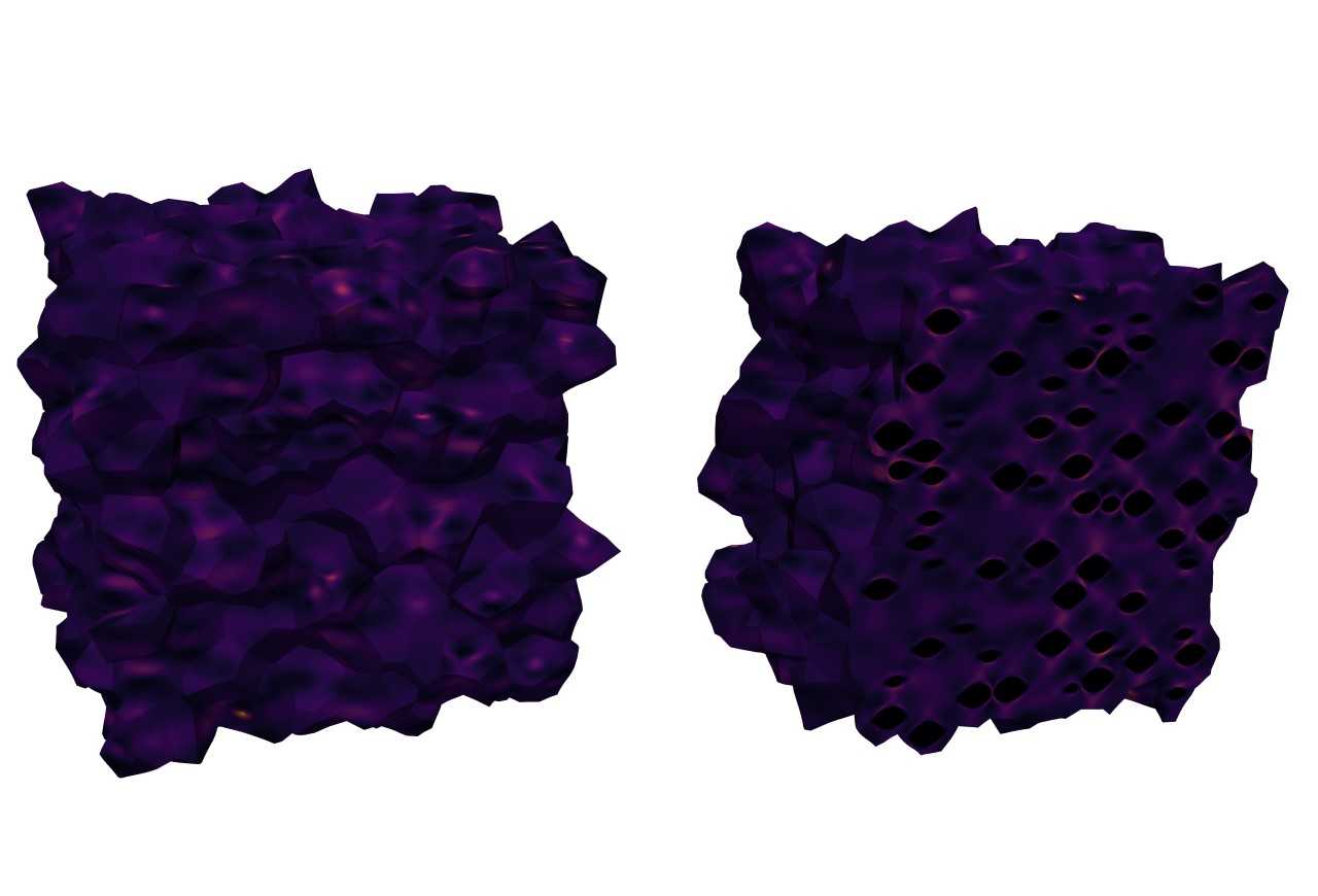
Benchmarks RVE MOX
In this section, we propose some scaling curves for different test cases. For the first benchmark, we use the MOX RVE example with 643 inclusions and a viscoplastic behavior law for the matrix, and an elastic behavior law for the inclusions. Calculations are performed on the TOPAZE supercomputer at CCRT. Each node in the cluster is built on 64-core AMD EPYC Milan 7763 dual-socket processors running at 2.45 GHz and equipped with 256 GB RAM. Benchmarks are in pure MPI.
Regarding the specificities of the simulations, we use the HyprePCG solver with a HypreBoomerAMG preconditioner. Mesh reading is performed using a mesh pre-cut into small msh files to limit the impact on the memory footprint.
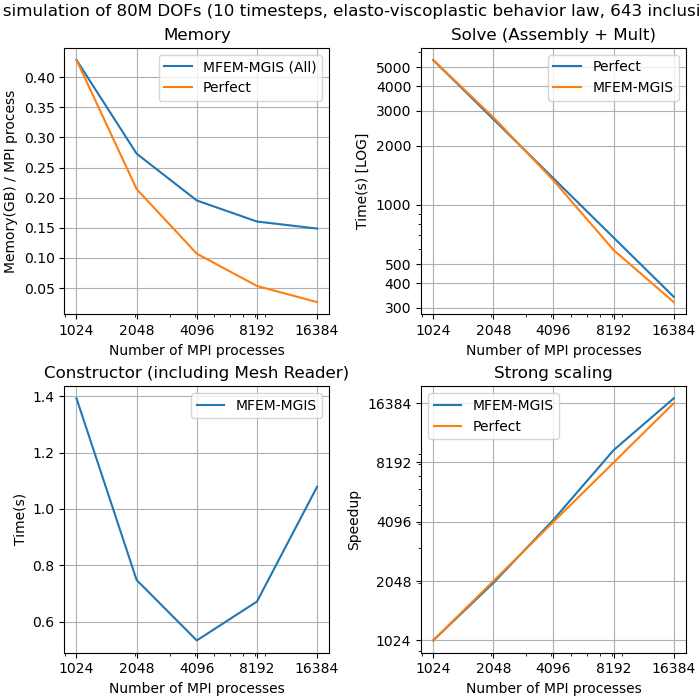
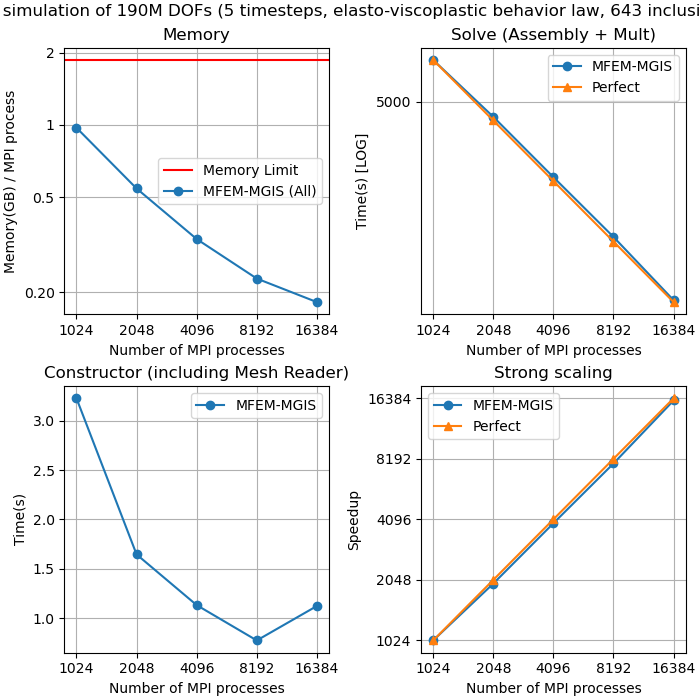
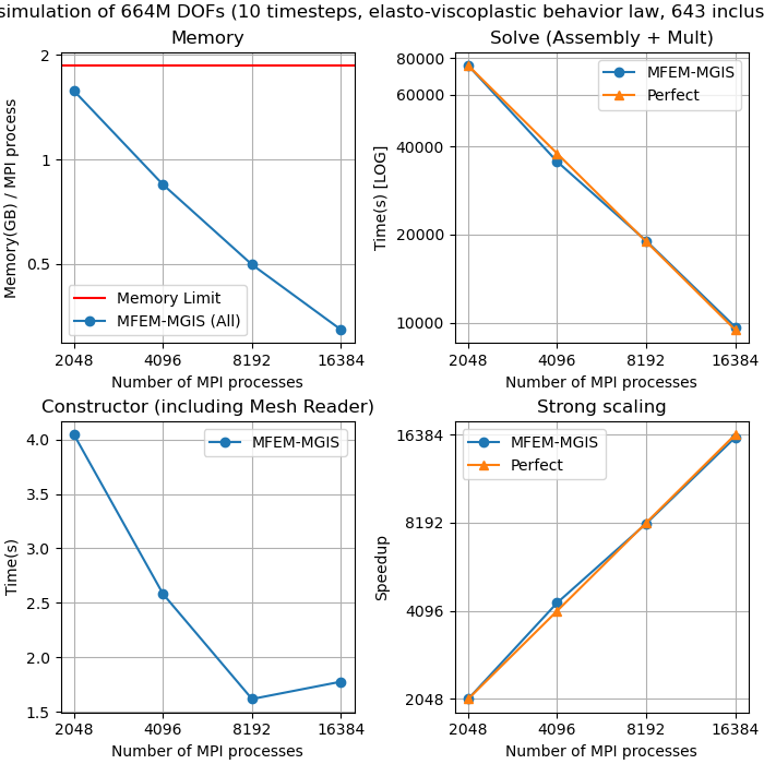
We performed tests on 3 problem sizes: 80M ddl, 190M ddl and 664M ddl.
Note
A feasibility test of this simulation was also carried out on more than 5.3 billion ddl.
80M ddl
190M ddl
664M ddl
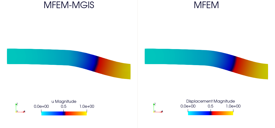
MFEM/MGIS versus MFEM
This benchmark aims to evaluate the time overhead between MFEM and MFEM/MGIS for a simple test case involving an elastic behavior law.
Details:
Solver: HyprePCG
Preconditioner: HypreDiagScale (Jacobi)
Tolerance: 1e-14
Boundary conditions: we impose a uniform Dirichlet condition U = (0,0,0) at left and U = (0,0,1) at right.
Refinement |
MPI |
DDL |
MFEM-MGIS Time |
MFEM-MGIS Iteration |
MFEM Time |
MFEM Iteration |
Overhead |
4 |
1 |
111843 |
8.34 |
1592 |
6.21 |
1565 |
34.4 % |
5 |
1 |
839619 |
122.54 |
3167 |
94.53 |
3102 |
29.6 % |
5 |
16 |
839619 |
51.34 |
3167 |
41.90 |
3102 |
22.5 % |
6 |
16 |
6502275 |
1057.24 |
6273 |
877.92 |
6124 |
20.0 % |
Note
Note that due to the small size of the input mesh, domain decomposition is limited to 16 subdomains (MFEM-MGIS only performs parallel refinement). To improve this benchmark, consider using sequential refinement or a finer mesh.
Run this example on Topaze supercomputer:
ccc_mprun -n 16 -c 1 -m work -T 600 -p milan -Q test ./MFEMLinearElasticityBenchmark --mesh ../beam-tet.mesh -r 5
ccc_mprun -n 16 -c 1 -m work -T 600 -p milan -Q test ./MFEMMGISLinearElasticityBenchmark --mesh ../beam-tet.mesh -r 5