Cermet simulation

Repository: https://github.com/rprat-pro/mm-opera-hpc/tree/main/cermet

Description

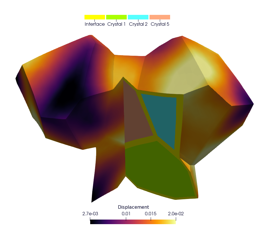
This case is similar to the UO2 polycrystal with the addition of a metallic interface at the grain boundary. In the Gmsh mesh each grain has a material ID (from 2 to \(N_{\text{grain}} + 1\)), as well as its orientation needed for the orthotropic basis. The metallic interface has the material ID equal to 1, and is considered to be made of an isotropic elasto-viscoplastic material. In addition to the mechanical analysis, this example implements a fixed-point algorithm enabling the simulation of a uniaxial compression/tensile test with periodic boundary conditions.

Parameters

• Boundary conditions: periodic boundary conditions are applied on the RVE faces. The loading is imposed in one direction, ensuring compatibility and equilibrium across periodic faces. More precisely, the axial component \(F_{zz}\) of the macroscopic deformation gradient is imposed. The off-diagonal components of the macroscopic deformation gradient are set to zero. The components \(F_{xx}\) and \(F_{yy}\) are the unknowns, determined via the fixed-point algorithm imposing null values for the components \(S_{xx}\) and \(S_{yy}\) of the macroscopic Cauchy stress tensor. The main result used for verification is a stress-strain curve with the evolution of the axial component \(S_{zz}\) of the Cauchy stress as a function of \(F_{xx}\).

• [Crystal] Constitutive law: The UO₂ crystal plasticity law used in the example is detailed in the reference [1]. The corresponding MFront file is available on the MMM GitHub repository. For uranium dioxide, the crystal symmetry is cubic, with the following orthotropic elastic properties:

  • Young’s modulus = \(222\times10^9\ \text{Pa}\)

  • Poisson ratio = 0.27

  • Shear modulus = \(54\times10^9\ \text{Pa}\)

• [Metallic Interface] Constitutive law: The Norton creep law used for the interface is derived from the elasto-viscoplastic properties of chromium coatings used in eATF claddings, as proposed in the literature. The corresponding MFront file is available on the MMM GitHub repository.

• Elastic properties: - Young’s modulus = \(276\times10^9\ \text{Pa}\) - Shear modulus = \(54\times10^9\ \text{Pa}\)

• Norton creep law:

  \[\dot{\varepsilon}_{eq} = \frac{A D_0 \exp\!\left(-\frac{Q}{R T}\right)}{b^2} \left( \frac{\sigma_{eq}}{C} \right)^n\]

  with the parameters:

  • \(A = 2.5\times10^{11}\) [a.u.]

  • \(n = 4.75\)

  • \(Q = 3.0627\times10^{5}\) [a.u.]

  • \(D_0 = 1.55\times10^{-5}\) [a.u.]

  • \(b = 2.5\times10^{-10}\) [a.u.]

• Finite element order: 1 (linear interpolation)

• Finite element space: H1

• Simulation duration: 200 s

• Number of time steps: 500

• Linear solver: HyprePCG (solver / preconditioner)

Mesh generation

This section explains how to generate a sample mesh with Merope.

Before running the script, make sure that the environment variable MEROPE_DIR is properly loaded.

Then, you can generate the mesh in two steps:

source ${MEROPE_DIR}/Env_Merope.sh
python3 mesh/5grains.py    # generate 5grains.geo
gmsh -3 5grains.geo        # generate 5grains.msh

You will obtain a 3D mesh (5grains.msh) of a polycrystalline sample with 5 grains.

Options

Mesh Generation Examples

The mesh can be customized by adjusting the input parameters in the Python script.

Below are two examples:

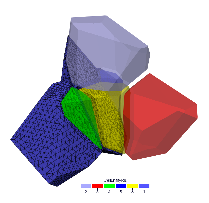
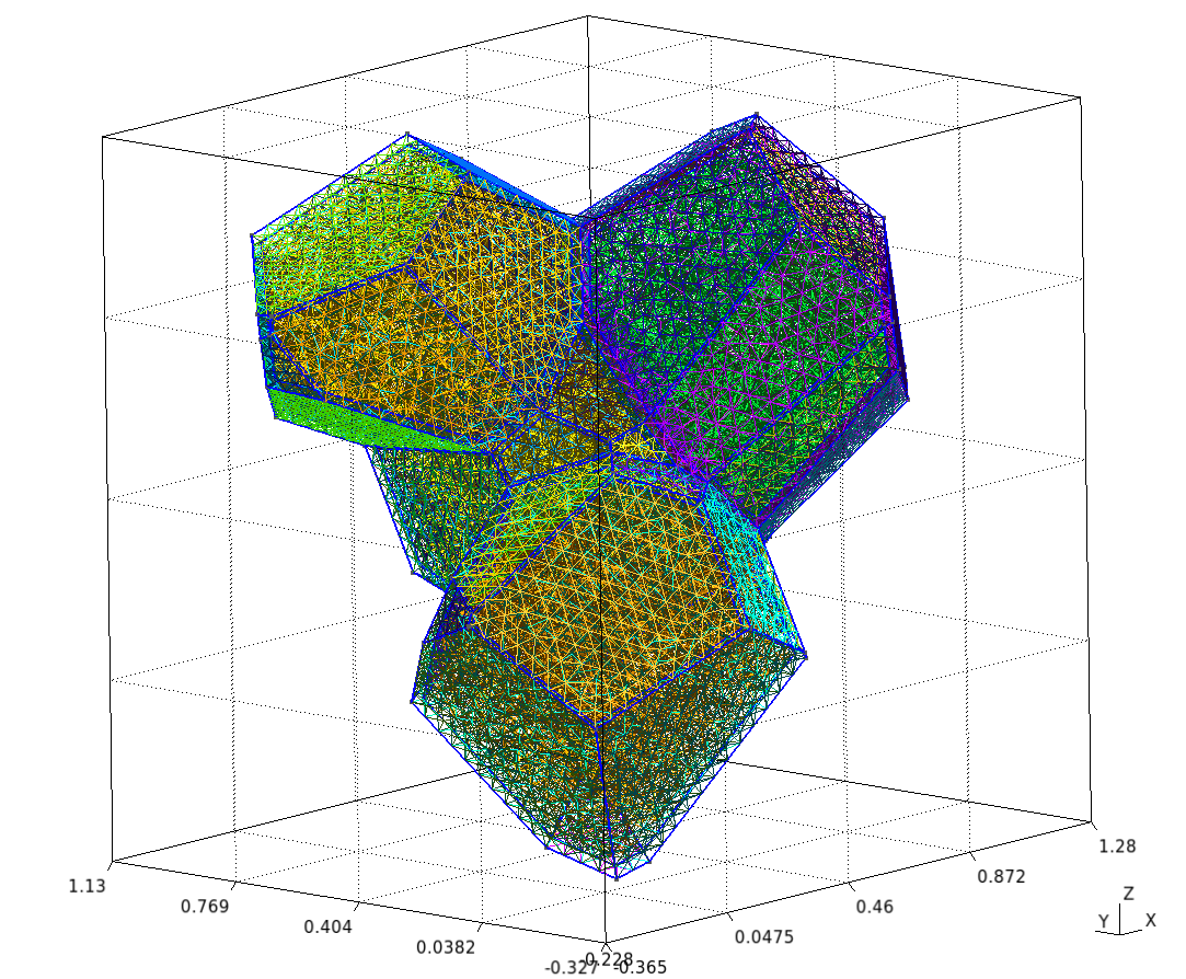
Small Example

This setup generates a small polycrystalline mesh (Gmsh version 11.1):

• 5 grains

• 12,992 nodes

• 88,687 elements

L = [1, 1, 1]
nbSpheres = 20
distMin = 0.3
randomSeed = 0
layer = 0.02
MeshOrder = 1
MeshSize = 0.05

Large Example

This setup generates a realistic polycrystalline mesh with:

• 250 grains

• 12,913,361 nodes

• 86,213,779 elements

L = [5, 5, 5]
nbSpheres = 250
distMin = 0.1
randomSeed = 0
layer = 0.04
MeshOrder = 1
MeshSize = 0.02

Run your simulation

Command-line Usage

Usage: ./cermet [options] ...

Option	Type	Default	Description
-h, --help	—	—	Print the help message and exit.
-m <string>, --mesh <string>	string	mesh/5grains.msh	Mesh file to use.
-o <int>, --order <int>	int	1	Finite element order (polynomial degree).
-r <int>, --refinement <int>	int	0	Refinement level of the mesh (default = 1).
-p <int>, --post-processing <int>	int	1	Run the post-processing step.
-v <int>, --verbosity-level <int>	int	0	Verbosity level of the output.
-d <double>, --duration <double>	double	200	Duration of the simulation (default = 5).
-n <int>, --nstep <int>	int	400	Number of simulation steps (default = 40).
-f <string>, --file <string>	string	vectors_5grains.txt	Vector file to use.
--macroscopic-stress-output-file <string>	string	cermet.res	Main output file containing: - Evolution of the diagonal components of the deformation gradient. - Evolution of the diagonal components of the Cauchy stress.

How to Run it

You can run the simulation in parallel using MPI. Below are two examples.

Basic Test

Runs a short simulation with:

• Duration = 0.5 s

• 1 timestep

• Mesh = 5grains.msh

• Refinement level = 0

mpirun -n 12 ./cermet --duration 0.5 --nstep 1

Full Test

Runs a longer simulation with:

• Duration = 200 s

• 400 timesteps

• Custom mesh (yourmesh.msh)

• Refinement level = 1

mpirun -n 12 ./cermet --duration 200 --nstep 400 -r 1 --mesh yourmesh.msh

Results

By default, the simulation generates the file cermet.res when running:

mpirun -n 12 ./cermet

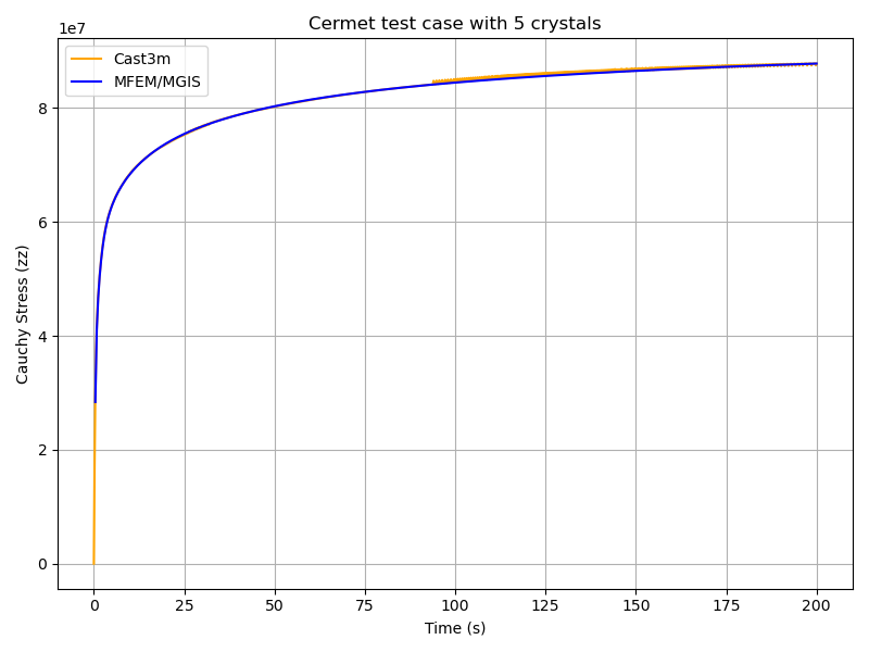
To validate the results, the Cauchy stress component in the z-direction (\(\overline{\sigma}_{zz}\)) can be compared with reference values obtained from Cast3M.

Plot and Compare

To visualize and compare the results, run the following Python script:

python3 plot_cermet_results.py

This script generates a figure named plot_cermet.png as shown below. In this figure, we observe good agreement between Cast3M and MFEM-MGIS results. As observed for the polycrystal test case, there are some oscillations in the Cast3M solution, which is of poorer quality compared to the MFEM-MGIS results. The main conclusion is that the implicit formulation of MFEM-MGIS (full Newton algorithm using the tangent stiffness) is highly performant—thanks to quadratic convergence and parallelization—and provides a high-quality solution. For verification, the number of time steps has been significantly increased to minimize the oscillations observed in Cast3M.

Check the values

To verify the simulation results, run:

python3 check_cermet_restults.py

The expected output is: Check PASS.

Example of the detailed output:

       Time     MFEM/MGIS      CAST3M  RelDiff_% Status
0      0.4  2.837174e+07  29462000.0   3.842755     OK
1      0.8  4.101172e+07  41798000.0   1.917200     OK
2      1.2  4.674008e+07  47113000.0   0.797856     OK
3      1.6  5.042402e+07  50687000.0   0.521535     OK
4      2.0  5.321536e+07  53452000.0   0.444677     OK
..     ...           ...         ...        ...    ...
495  198.4  8.775101e+07  87802000.0   0.058103     OK
496  198.8  8.775917e+07  87724000.0  -0.040076     OK
497  199.2  8.776730e+07  87804000.0   0.041820     OK
498  199.6  8.777539e+07  87814000.0   0.043988     OK
499  200.0  8.778345e+07  87737000.0  -0.052917     OK

                        [500 rows x 5 columns]
                        Check PASS.

This table shows the comparison between the simulated Cauchy stress values and the reference Cast3M results, along with the relative difference and a status check.

References

[1]

Portelette, L., Amodeo, J., Madec, R., et al. Crystal viscoplastic modeling of UO₂ single crystal. Journal of Nuclear Materials, 510, 635–643 (2018).